[1] 4[1] 5865.327Introduction to toolkit
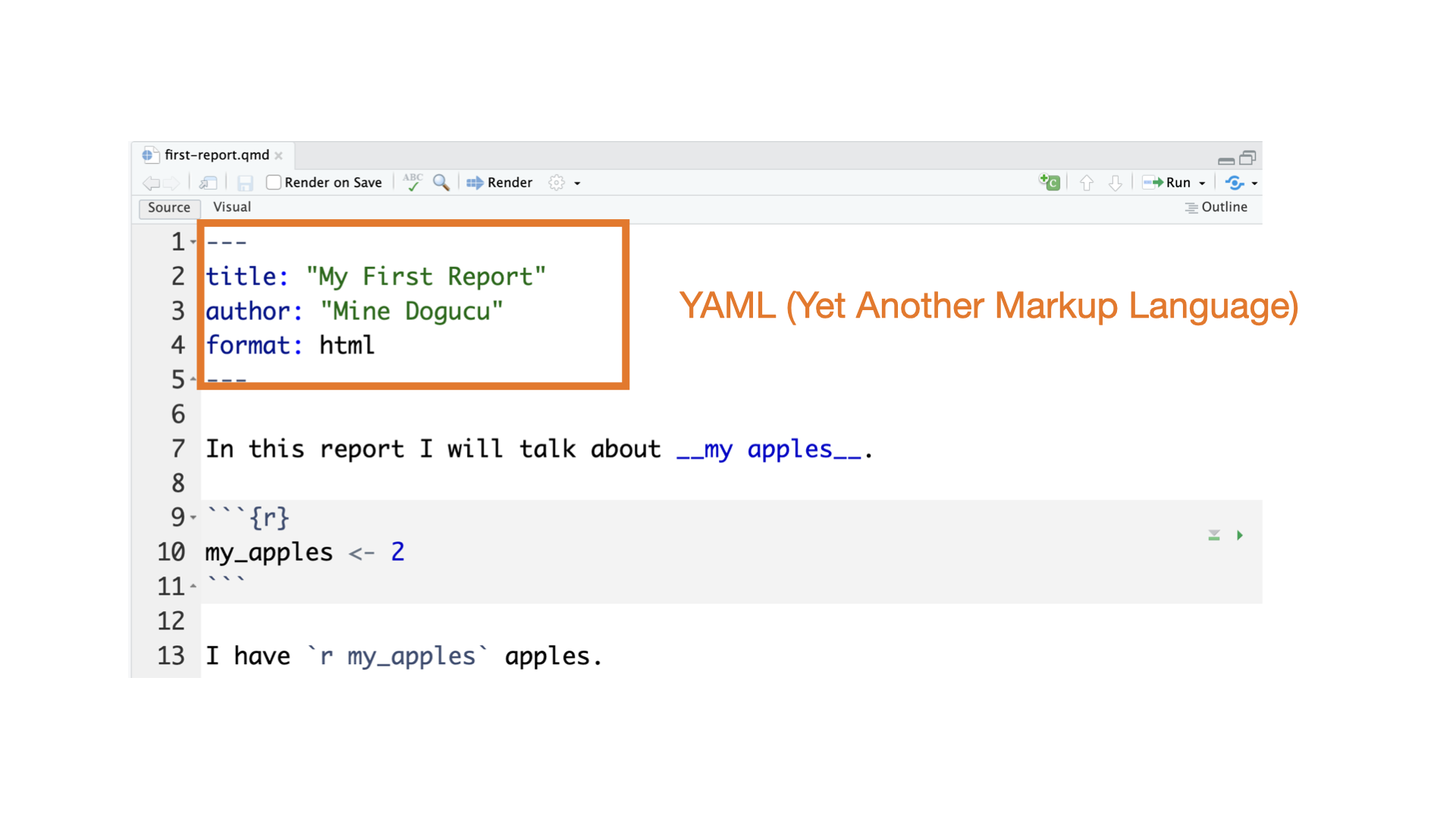
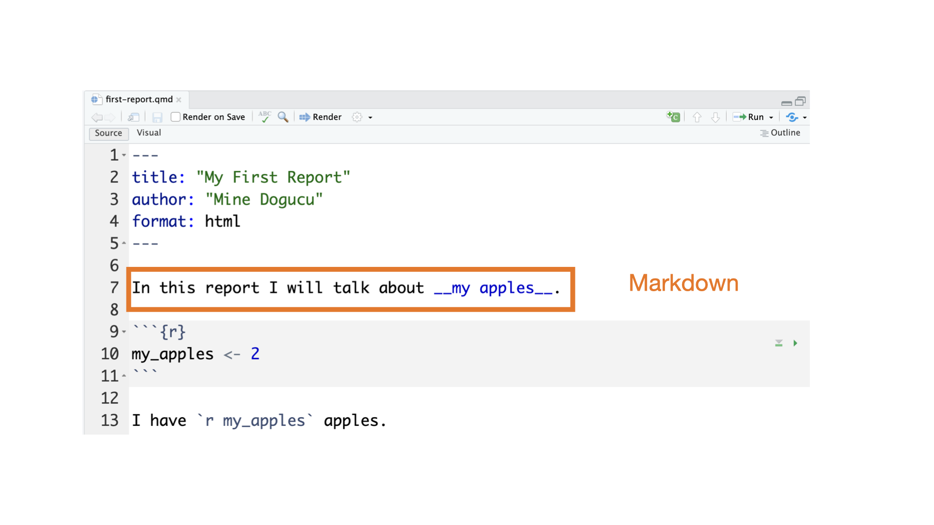
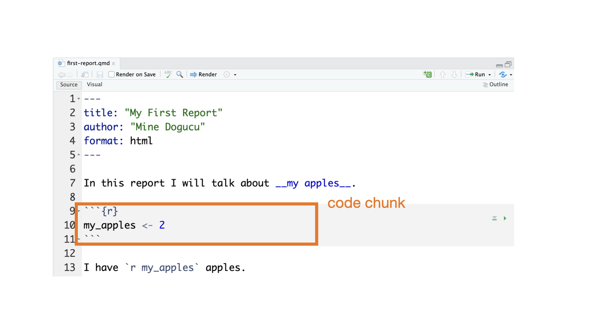
What you see is
We can save things into an object using the assignment operator <-
I can name it almost whatever I wish
Names of objects:
You can view what is in an object
R is case sensitive
Tip
Let R autocomplete for you to avoid spelling mistakes
Objects can store vectors also
We can also do elementwise math with vectors
The most common object type we will use are data frames
do() is a function;
something is the argument of the function.
Sometimes you may only want to specify one argument
Sometimes you want to provide multiple arguments
    One Sample t-test

data:  my_data
t = 6.4362, df = 7, p-value = 0.0003549
alternative hypothesis: true mean is not equal to 0
95 percent confidence interval:
 2.767658 5.982342
sample estimates:
mean of x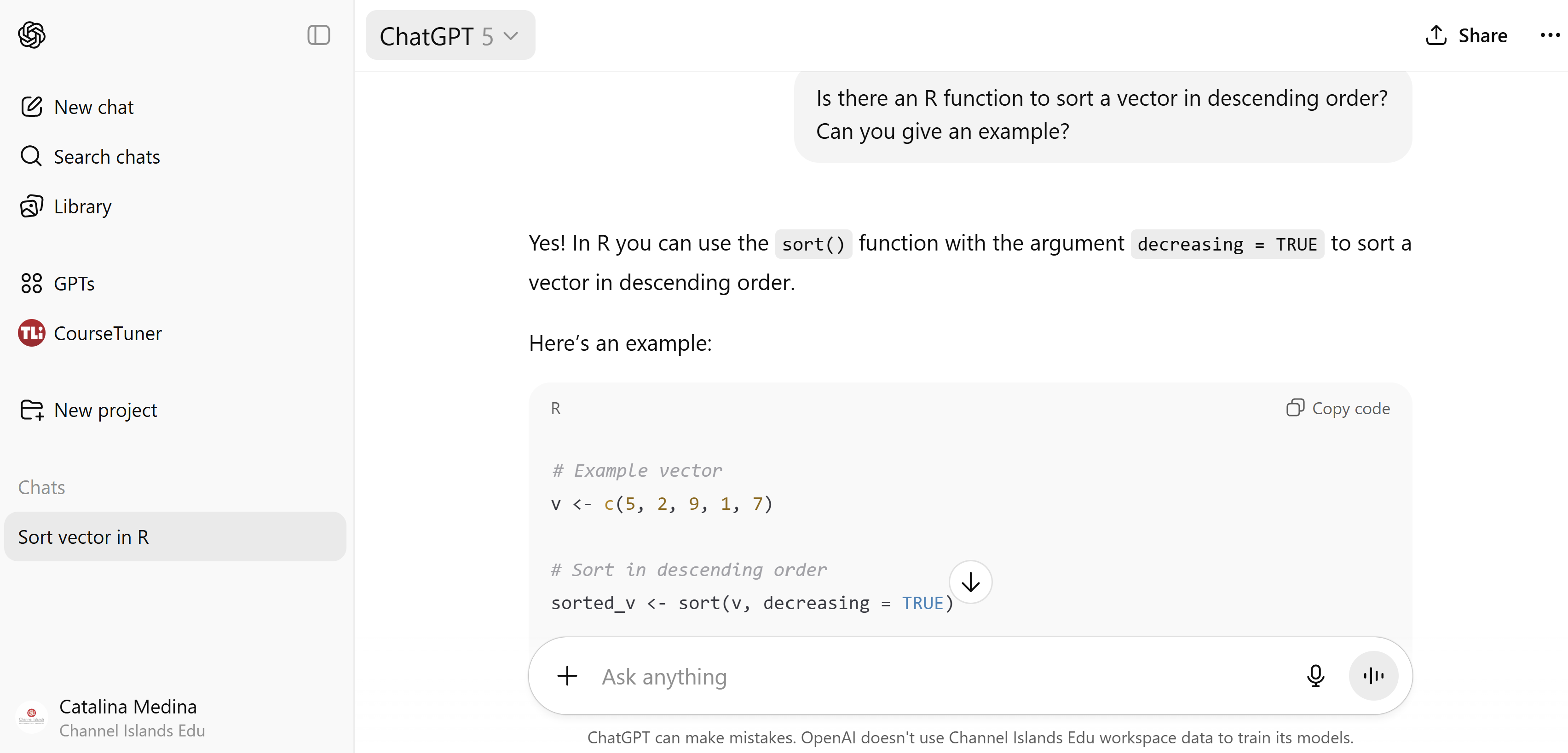
4.375 In order to get any help we can use ? followed by function (or object) name.
Tip
AI tools can be helpful for finding functions and providing examples.
Warning
You should not copy paste code from my slides or from the internet. Part of learning to code is building up your muscle memory.
Do not assume that AI tools will be correct. Even if the code runs it may not be the proper way of doing something.
If the code example is very long or does not use functions we discussed in class, refine your question.
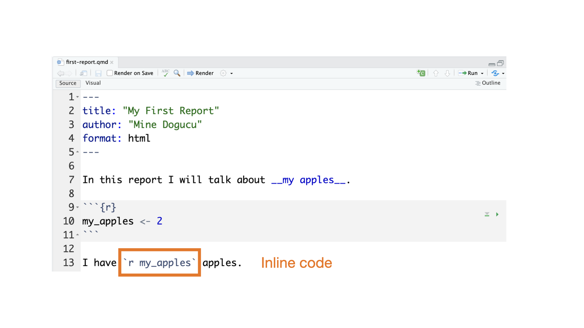
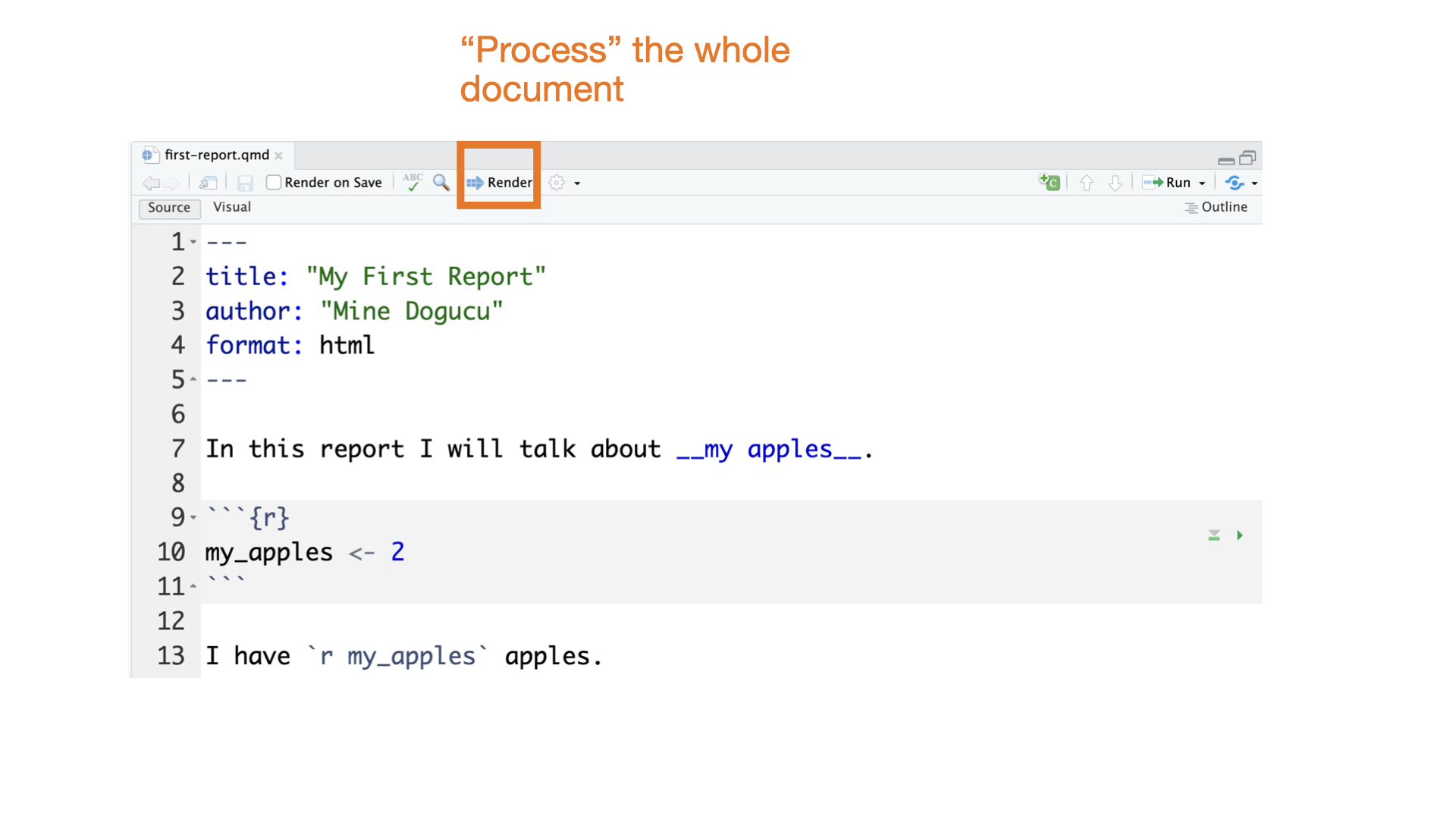
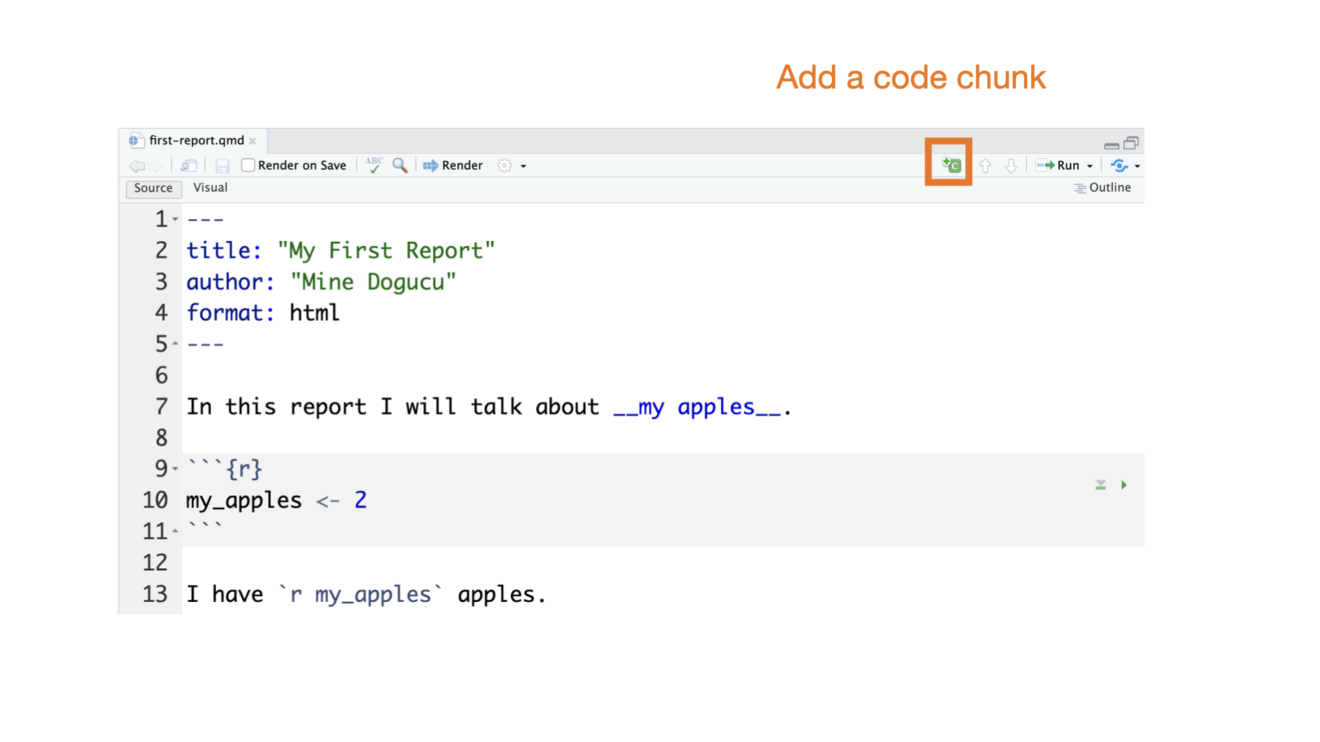
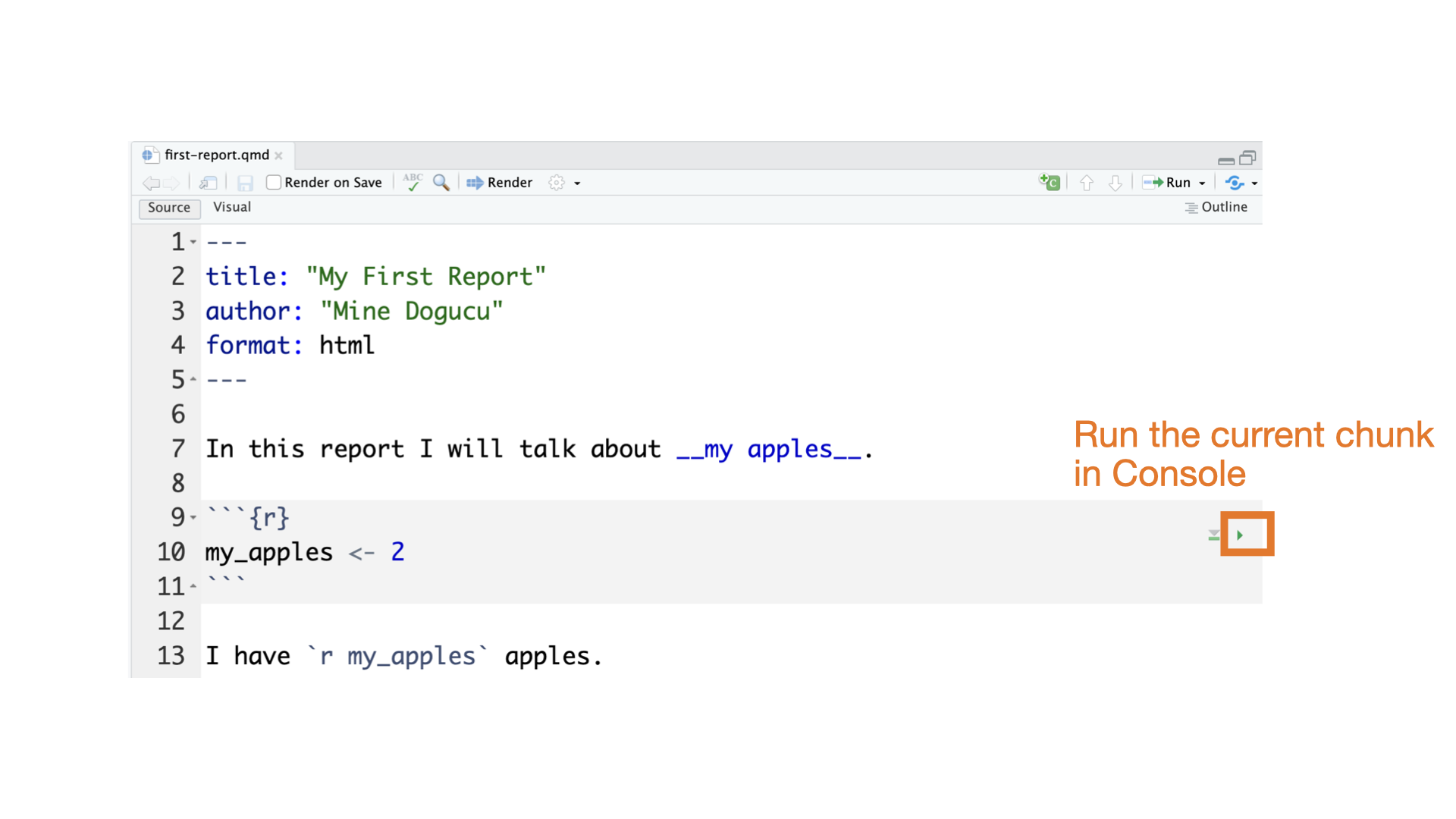
Slides that you are currently looking at are also written in Quarto. You can take a look at them on in the GitHub repository I use to make the slides.
When you buy a new phone it comes with some apps pre-installed.
If you want to use a different app you can install it.
When you download R for the first time to your computer. It comes with some packages already installed. You can also install many other R packages.
What do R packages have? All sorts of things but mainly
functions
datasets
In order to use a package you have to:
Try running the following code and look at the error:
The function beep() is from the beepr package, so we have to (1) make sure it is installed and then (2) load it
Dear Mona, Which State Has the Worst Drivers?
When you are given some code like this one in your lecture notes or assignments, you should run it first before beginning to code. As we progress in the course, you’ll have a deeper understanding of what the starter codes do.
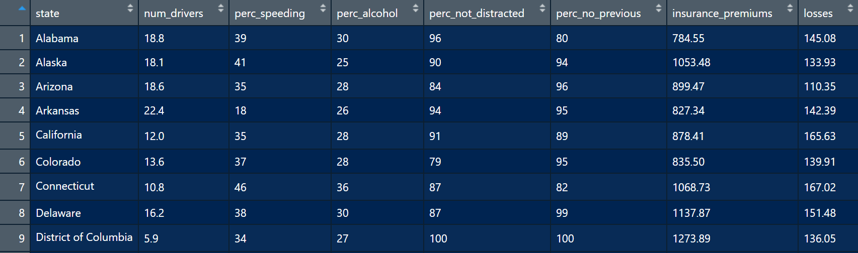
The data frame has 8 variables (state, num_drivers, perc_speeding, perc_not_distracted, perc_no_previous, insurance_premiums, losses).
The data frame has 51 cases or observations. Each case represents a US state (or District of Columbia).
If a dataset is part of an R package you can look at its help documentation.
In general we use a data dictionary for information on a data set. The data dictionary at minimum should contain information describing each column in the data set.
# A tibble: 6 × 8
  state      num_drivers perc_speeding perc_alcohol perc_not_distracted
  <chr>            <dbl>         <int>        <int>               <int>
1 Alabama           18.8            39           30                  96
2 Alaska            18.1            41           25                  90
3 Arizona           18.6            35           28                  84
4 Arkansas          22.4            18           26                  94
5 California        12              35           28                  91
6 Colorado          13.6            37           28                  79
# ℹ 3 more variables: perc_no_previous <int>, insurance_premiums <dbl>,
# losses <dbl># A tibble: 6 × 8
state num_drivers perc_speeding perc_alcohol perc_not_distracted
<chr> <dbl> <int> <int> <int>
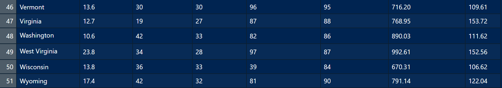
1 Vermont 13.6 30 30 96
2 Virginia 12.7 19 27 87
3 Washington 10.6 42 33 82
4 West Virginia 23.8 34 28 97
5 Wisconsin 13.8 36 33 39
6 Wyoming 17.4 42 32 81
# ℹ 3 more variables: perc_no_previous <int>, insurance_premiums <dbl>,
# losses <dbl>Rows: 51
Columns: 8
$ state <chr> "Alabama", "Alaska", "Arizona", "Arkansas", "Calif…
$ num_drivers <dbl> 18.8, 18.1, 18.6, 22.4, 12.0, 13.6, 10.8, 16.2, 5.…
$ perc_speeding <int> 39, 41, 35, 18, 35, 37, 46, 38, 34, 21, 19, 54, 36…
$ perc_alcohol <int> 30, 25, 28, 26, 28, 28, 36, 30, 27, 29, 25, 41, 29…
$ perc_not_distracted <int> 96, 90, 84, 94, 91, 79, 87, 87, 100, 92, 95, 82, 8…
$ perc_no_previous <int> 80, 94, 96, 95, 89, 95, 82, 99, 100, 94, 93, 87, 9…
$ insurance_premiums <dbl> 784.55, 1053.48, 899.47, 827.34, 878.41, 835.50, 1…
$ losses <dbl> 145.08, 133.93, 110.35, 142.39, 165.63, 139.91, 16…Import
Export
Tip
A lot of headaches can be prevented from using read_csv() instead of read.csv()!