We said our theoretical model is \[Y_i = \beta_0 + \beta_1 X_i + \epsilon_i.\]
It is theoretical because we are saying if we had all of the data for our population, a census instead of a sample, it would be the best linear approximation for the relationship between \(X\) and \(Y\).
Realistically we will almost never have a census, so \(\beta_0\) and \(\beta_1\) are unknown in practice.
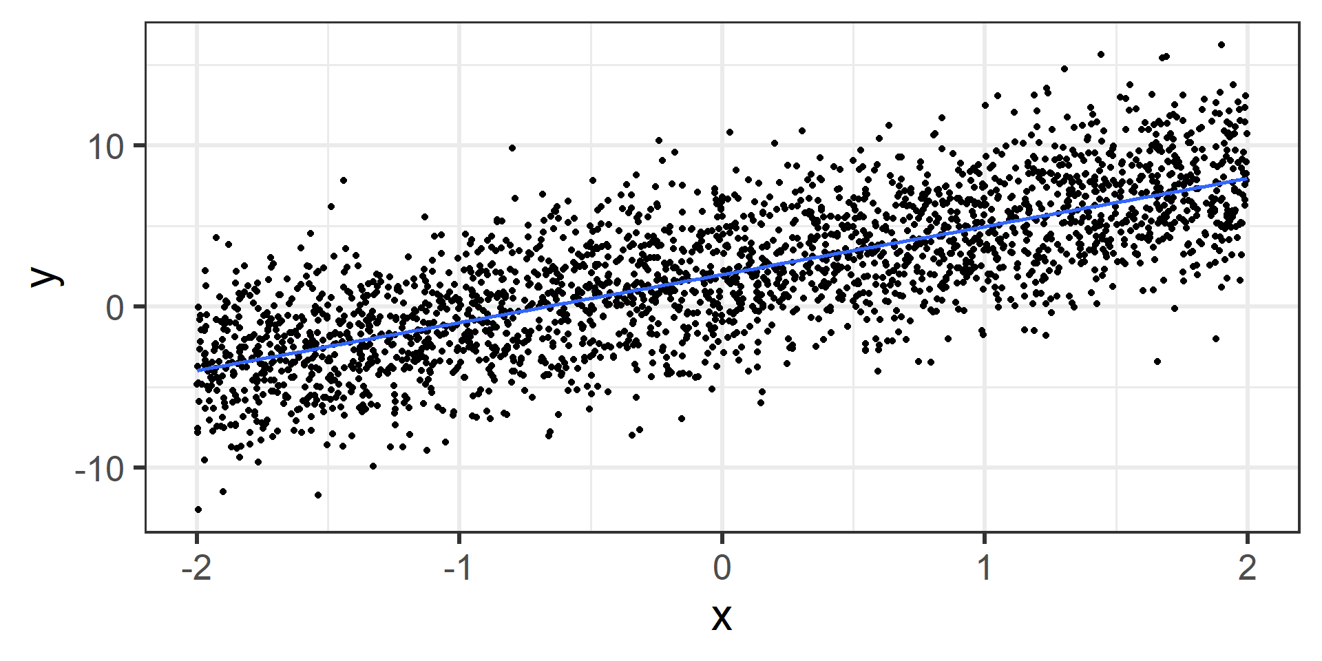
Simulation: population data
I simulated data for a population of 2500 individuals.
randomly generate \(x\)’s (doesn’t matter how).
randomly generate \(\epsilon\)’s where \(\epsilon_i \overset{iid}{\sim} N(0, 3^2)\).
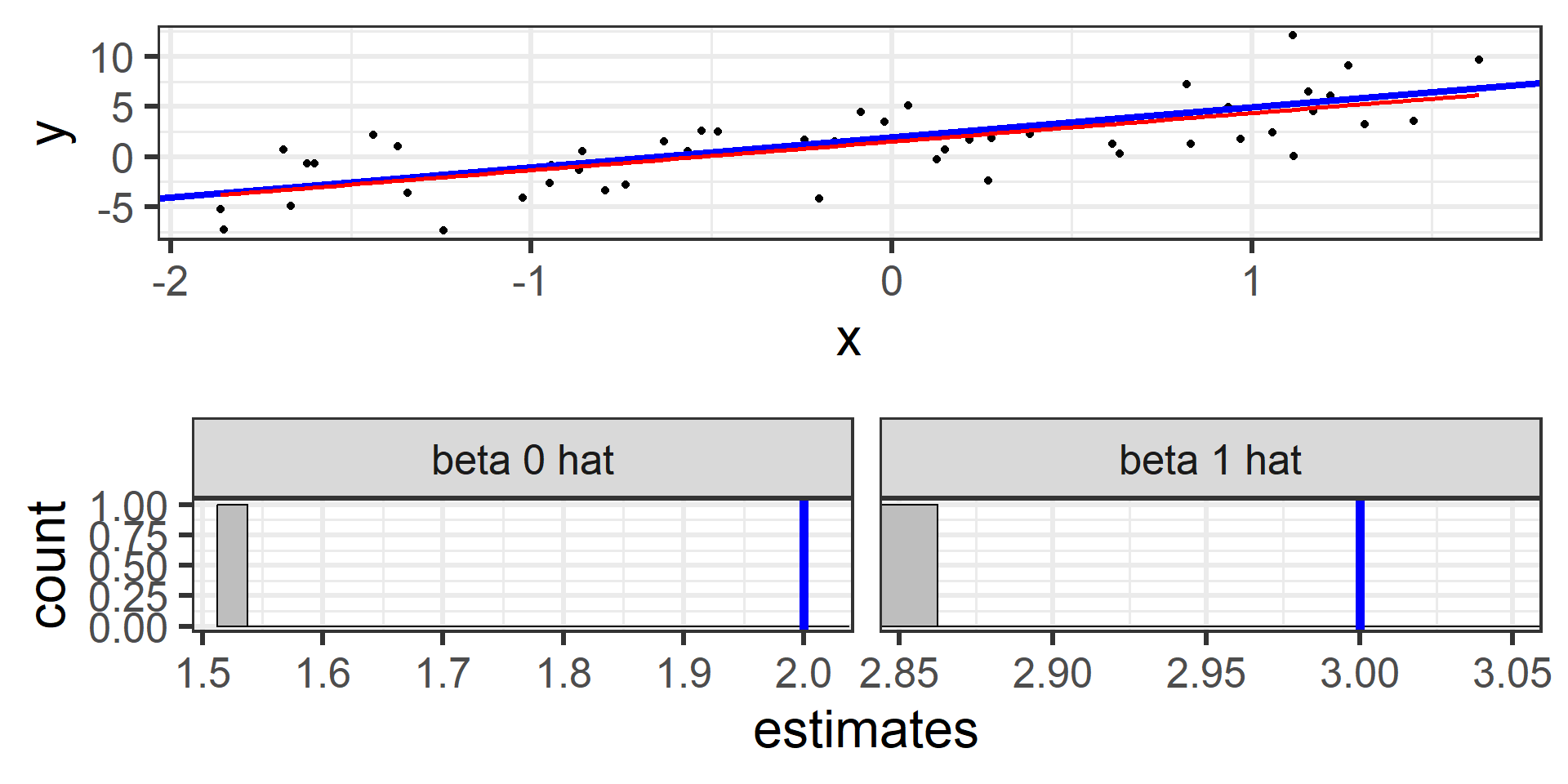
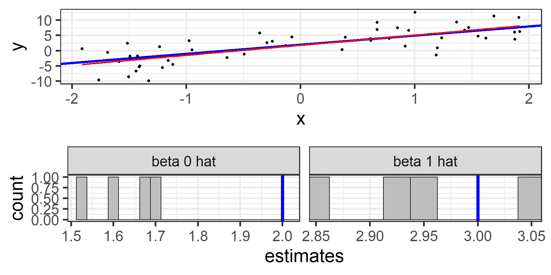
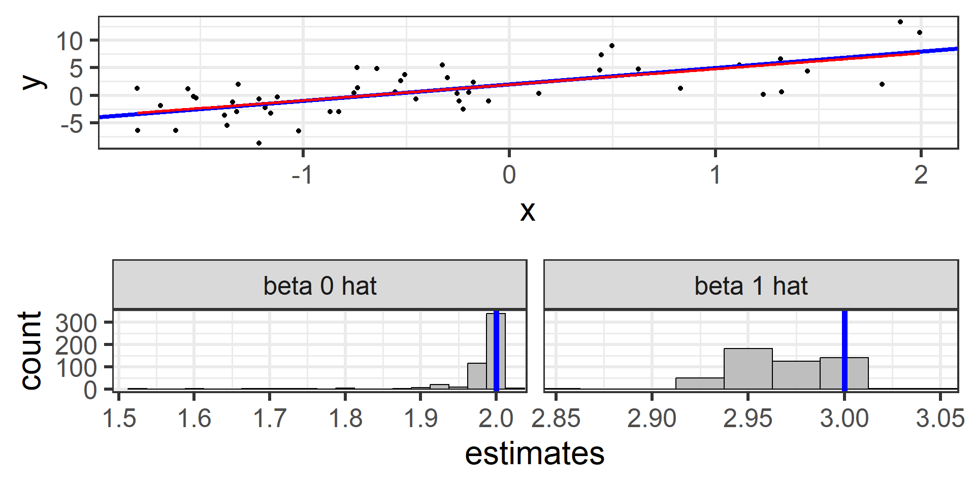
Next I randomly sampled 50 individuals and calculate the least squares estimates \(\hat{\beta}_0\) and \(\hat{\beta}_1\)
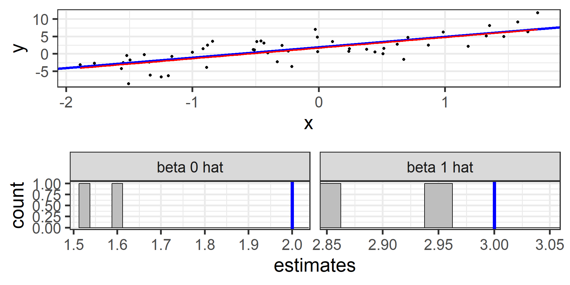
Simulation: simple random sample 2
I can do that again with another random sample of 50.
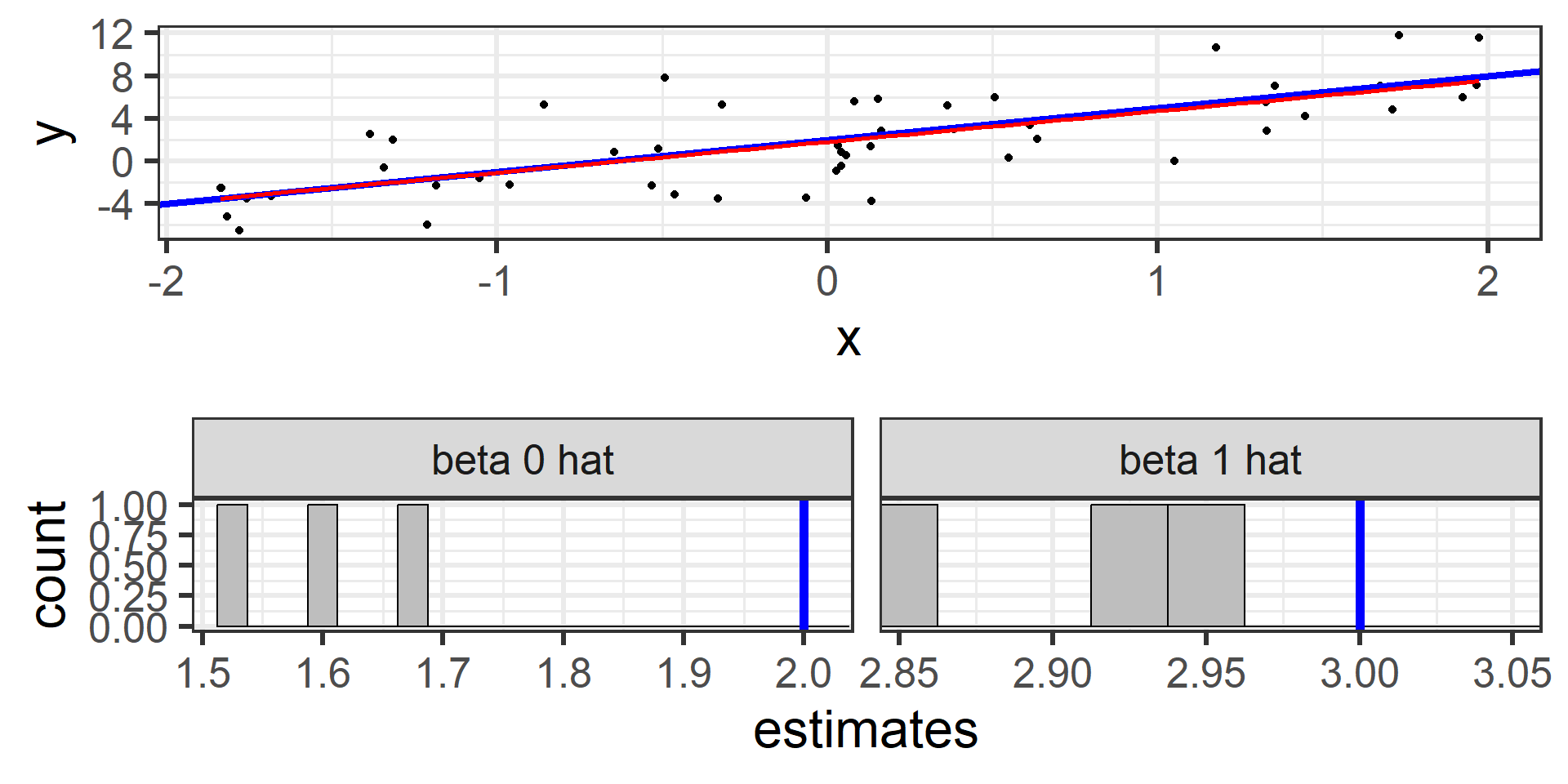
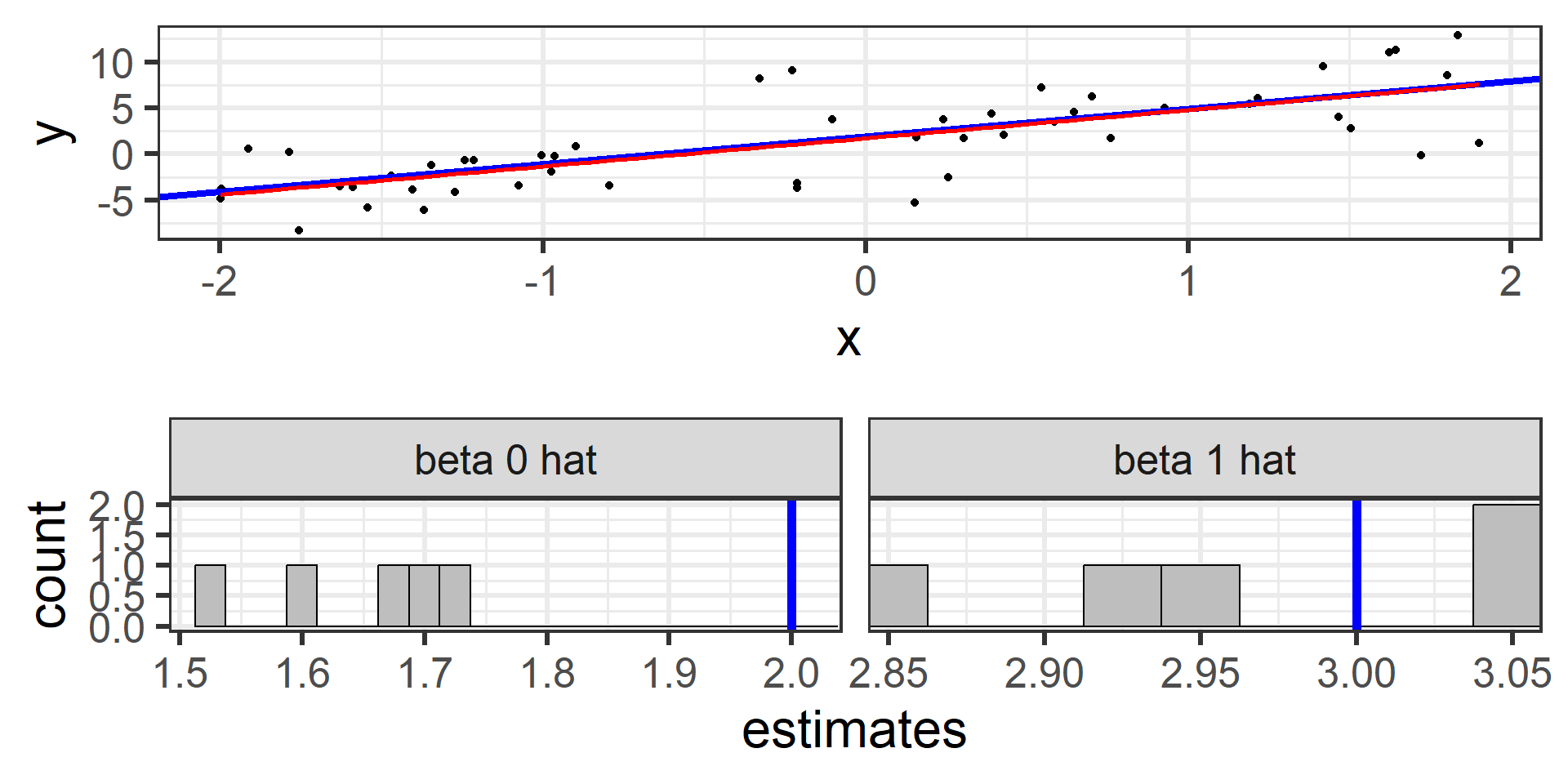
Simulation: simple random sample 3
And again with a third random sample of 50
Simulation: simple random sample 4
And again with a fourth random sample of 50
Simulation: simple random sample 5
And again with a fifth random sample of 50
Simulation: simple random sample 50
And again 50 times!
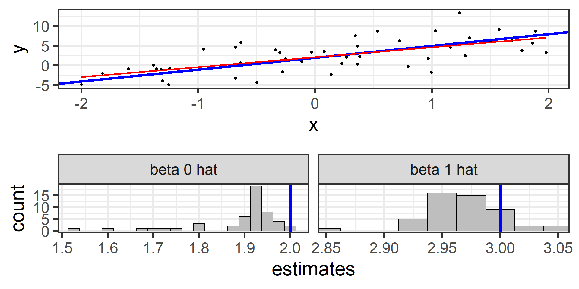
Simulation: simple random sample 100
100 times!
Simulation: simple random sample 500
500 times!
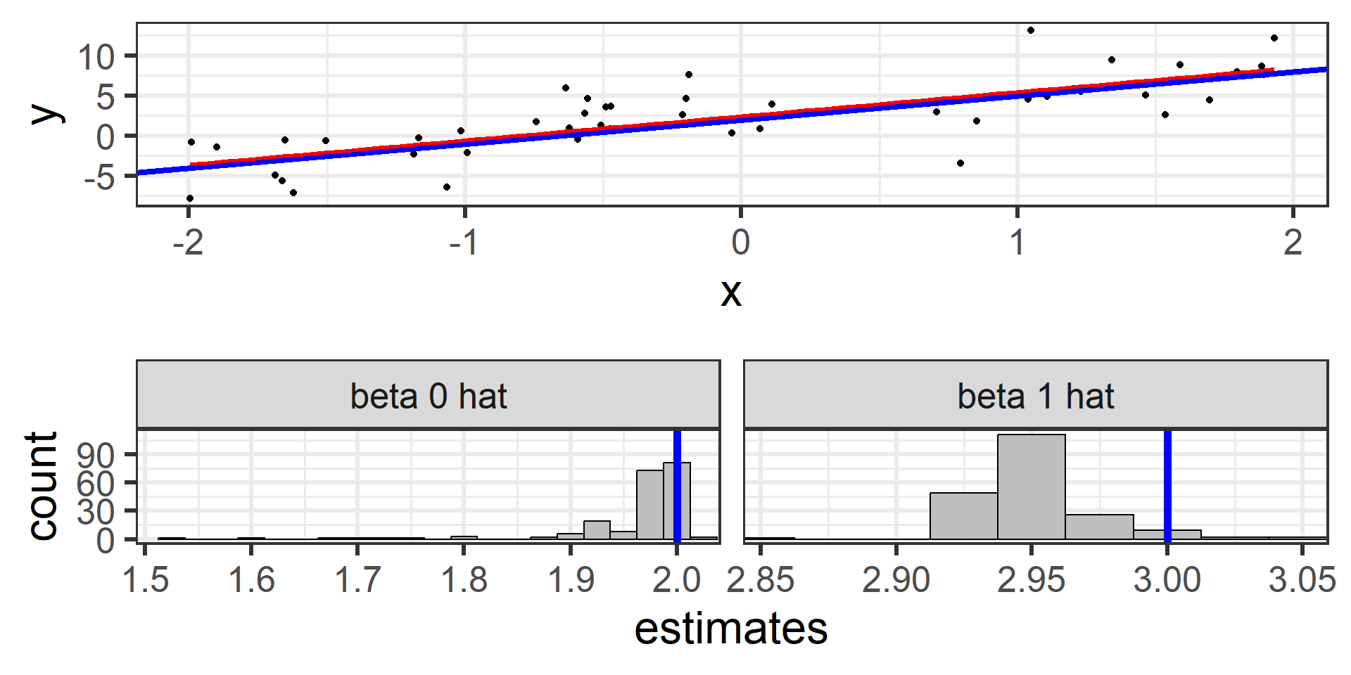
Simulation: simple random sample 1000
Even 1000 times!
Unbiased estimators
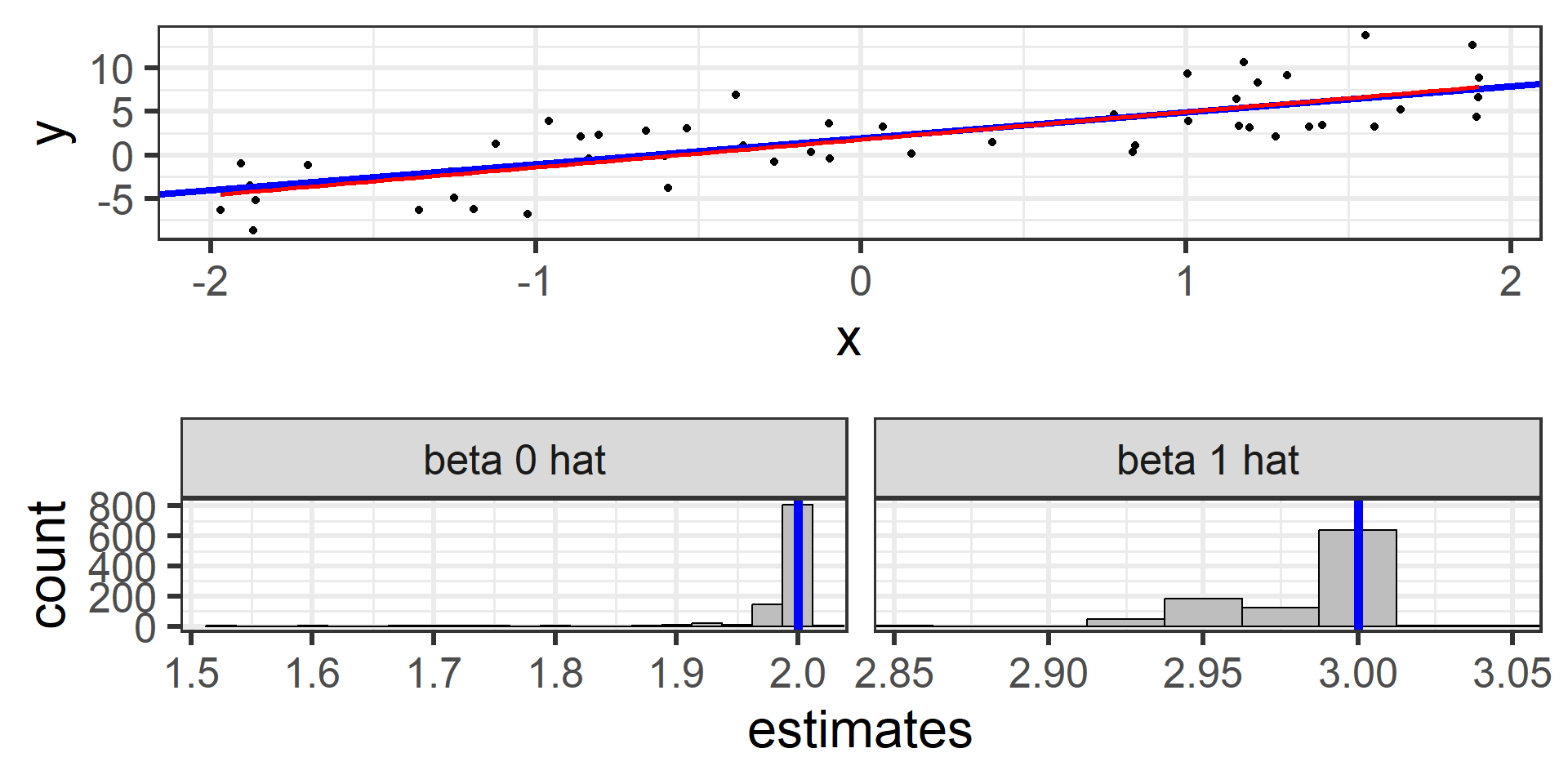
What we just saw was the sampling distribution of \(\hat{\beta}_0\) and \(\hat{\beta}_1\).
The least squares estimators \(\hat{\beta}_0\) and \(\hat{\beta}_1\) from many random samples will tend towards the true parameters \(\beta_0\) and \(\beta_1\).
\(\hat{\beta}_0\) and \(\hat{\beta}_1\) are unbiased estimators for \(\beta_0\) and \(\beta_1\)! \(E[\hat{\beta}_0] = \beta_0\) and \(E[\hat{\beta}_1] = \beta_1\)
In practice we typically only have one sample and the estimates from a single sample may be fairly different from the true parameters by chance.
This is why we should use uncertainty estimates when using our estimators!
Technically what we calculate are estimates of the uncertainty estimators: \(\hat{SE(\hat{\beta}_0)}\) and \(\hat{SE(\hat{\beta}_1)}\)
SE and RSE in model output
elephant_model <-lm(Mass ~ Height, data = elephants)summary(elephant_model)
Call:
lm(formula = Mass ~ Height, data = elephants)

Residuals:
     Min       1Q   Median       3Q      Max
-1375.40  -193.73   -32.32   153.63  1457.10

Coefficients:
              Estimate Std. Error t value Pr(>|t|)
(Intercept) -3553.9303   111.5451  -31.86   <2e-16 ***
Height         27.1575     0.4885   55.59   <2e-16 ***
---
Signif. codes:  0 '***' 0.001 '**' 0.01 '*' 0.05 '.' 0.1 ' ' 1

Residual standard error: 305.3 on 1468 degrees of freedom
Multiple R-squared:  0.6779,    Adjusted R-squared:  0.6777
F-statistic:  3090 on 1 and 1468 DF,  p-value: < 2.2e-16
Confidence Intervals
Confidence interval formula
We can use our point estimates \(\hat{\beta}_0\) and \(\hat{\beta}_1\) along with our standard error estimates \(SE(\hat{\beta}_0)\) and \(SE(\hat{\beta}_1)\) to provide confidence intervals
For hypotheses tests we assume the null is true (\(H_0\)), and see if we can find evidence against it (i.e., low p-value), in support of the alternative hypothesis (\(H_1\))