Math 430: Lecture 5a

Linear Regression Conditions

Professor Catalina Medina

We discussed how simple linear regression can be used to solve different goals

Prediction

• We want the fitted line so we can use it on future data

Inference

• Learn the relationship between \(Y\) and \(X\) (confidence interval)
• Test if there is a linear relationship between \(Y\) and \(X\) (hypothesis test)

Recall our linear regression from last week

ggplot(elephants, aes(x = Height, y = Mass)) +
  geom_point() +
  geom_smooth(method = "lm", se = FALSE) +
  labs(x = "Height (cm)", y = "Mass (kg)")

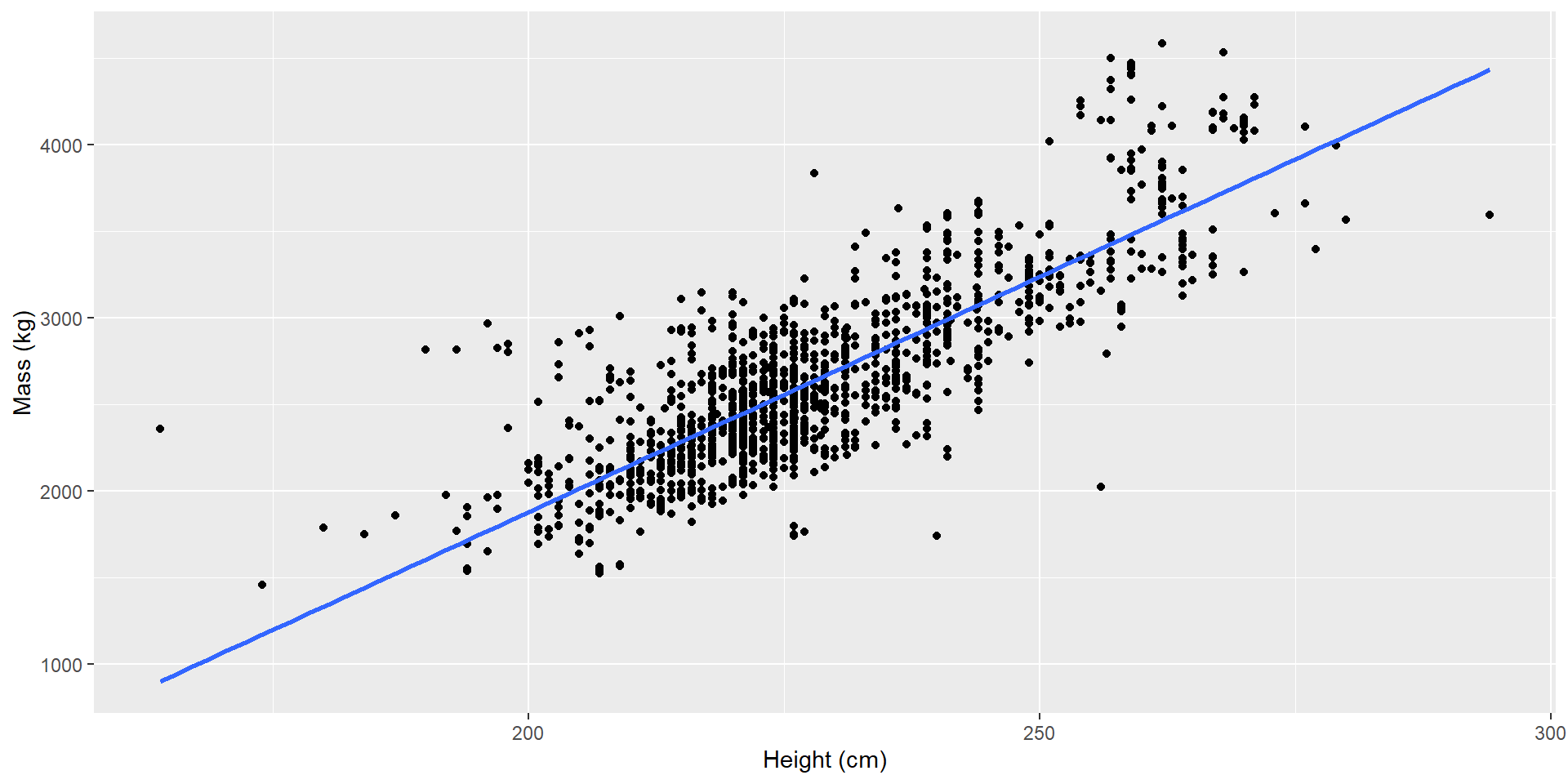
Was this model appropriate?

Why would we care if the model is “appropriate”?

• it may be chance that we got a good fit for our sample, but the model might be a bad fit for the population
• our estimates relied on our conditions, so if those don’t hold our estimates are meaningless

Conditions

\[Y_i = \beta_0 + \beta_1 X_i + \epsilon_i, \epsilon_i \overset{iid}{\sim} N(0, \sigma^2)\]

In order of importance:

1. Linearity: Linear relationship between \(X\) and \(Y\) (\(E[\epsilon_i] = 0)\).
2. Independence: Independence of \(\epsilon_i\).
3. Homoskedasticity: Constant variance of \(\epsilon_i\).
4. Normality: Normally distributed \(\epsilon_i\).

Checking model conditions

Visual checks versus statistical tests

People have developed some statistical tests to asses some model conditions.

• We want to avoid unnecessary tests because each test we perform introduces some error.

Alternatively, we will use visual assessments

• There is some level of subjectivity
• We will use experience and reproducibility to be responsible

Visual checks

model_elephant <- lm(Mass ~ Height, data = elephants)

library(ggfortify)

autoplot(model_elephant)

Recall residuals: \(e_i = y_i - \hat{y}_i\)

Visual checks

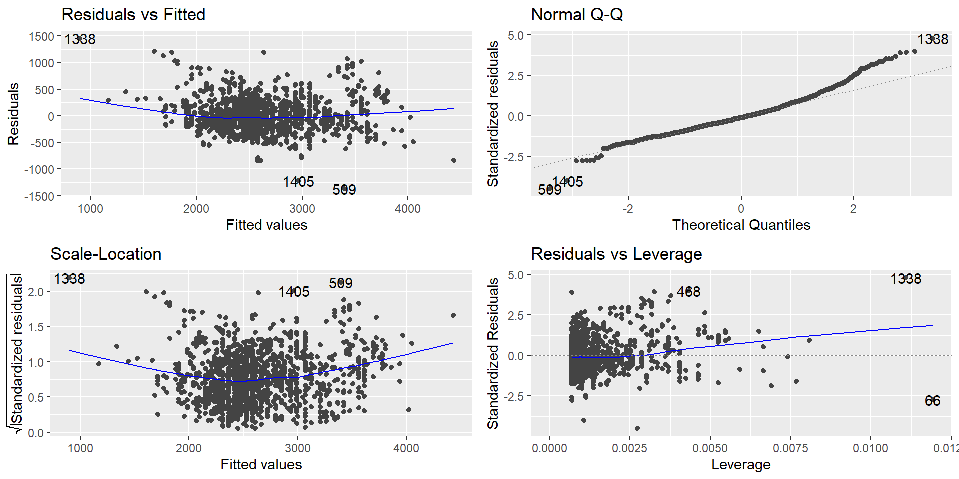
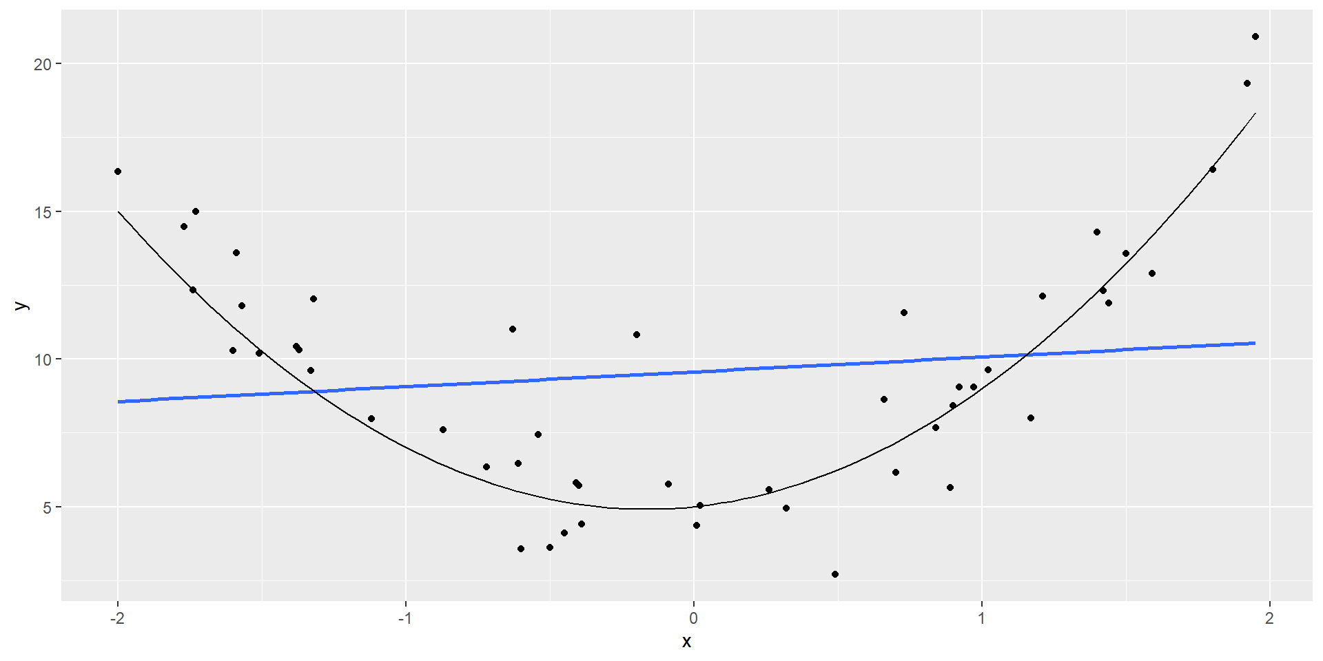
Diagnosing linearity

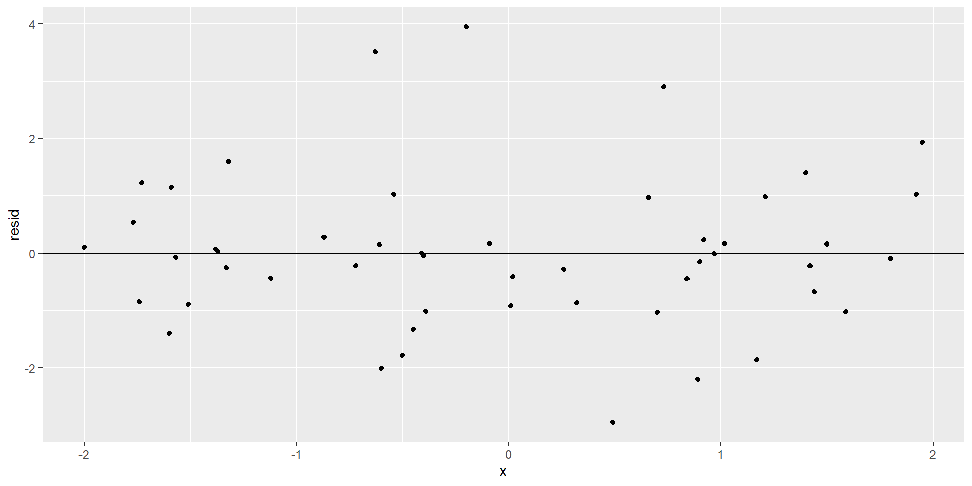
• Examine plot of residuals vs fitted (or predictor for simple linear regression)
• There should be no discernible pattern the the residuals centered around 0

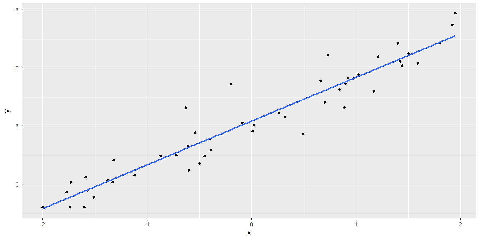
Linear

Non-linear

When linearity is violated

Implications:

• poor fit
• biased inference

Remedy:

• consider transformations of \(X\) or other relationships

Diagnosing Independence

• Consider how the data were collected (random sample? no repeat sampling?) and on whom the data were collected (would you expect independence?)
• Dependence could be revealed by plotting residuals versus unmodeled variables (time, class, etc)

When independence is violated

Implications:

• Estimators \(\hat{\beta}_0\) and \(\hat{\beta}_1\) are still unbiased
• The standard errors will underestimate the true standard errors
• Increased type one error rates (false positive)

Remedy:

• Consider a different model that accounts for correlation (e.g. if you have longitudinal data then a linear mixed effects model may be appropriate)

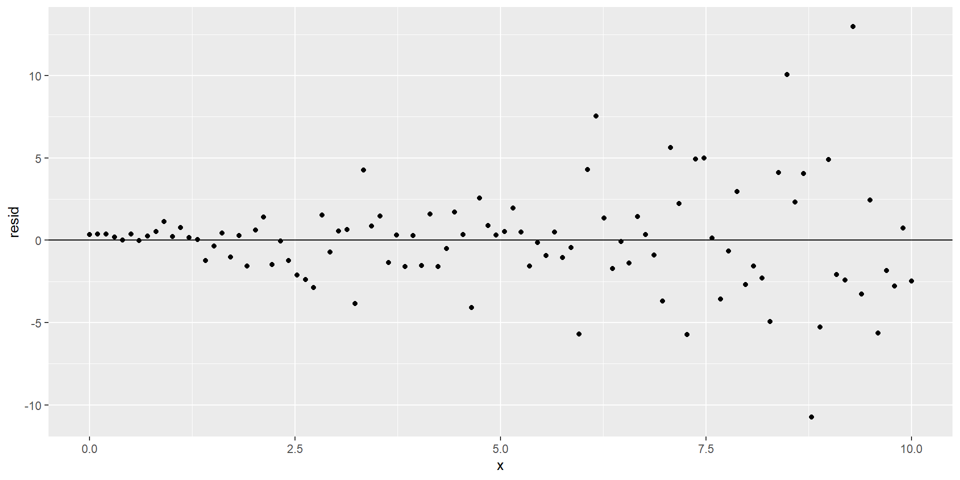
Diagnosing homoskedasticity

• Examine plot of residuals vs fitted and check there is not a “funnel-shape”
• Specifically, for each fitted value does the spread of the residuals look similar?

Constant variance

Non-constant variance

When homoskedasticity is violated

Implications:

• Estimators \(\hat{\beta}_0\) and \(\hat{\beta}_1\) are still unbiased
• The standard errors are incorrect

Remedies:

• Consider transformations of \(Y\)
• Consider Weighted least squares

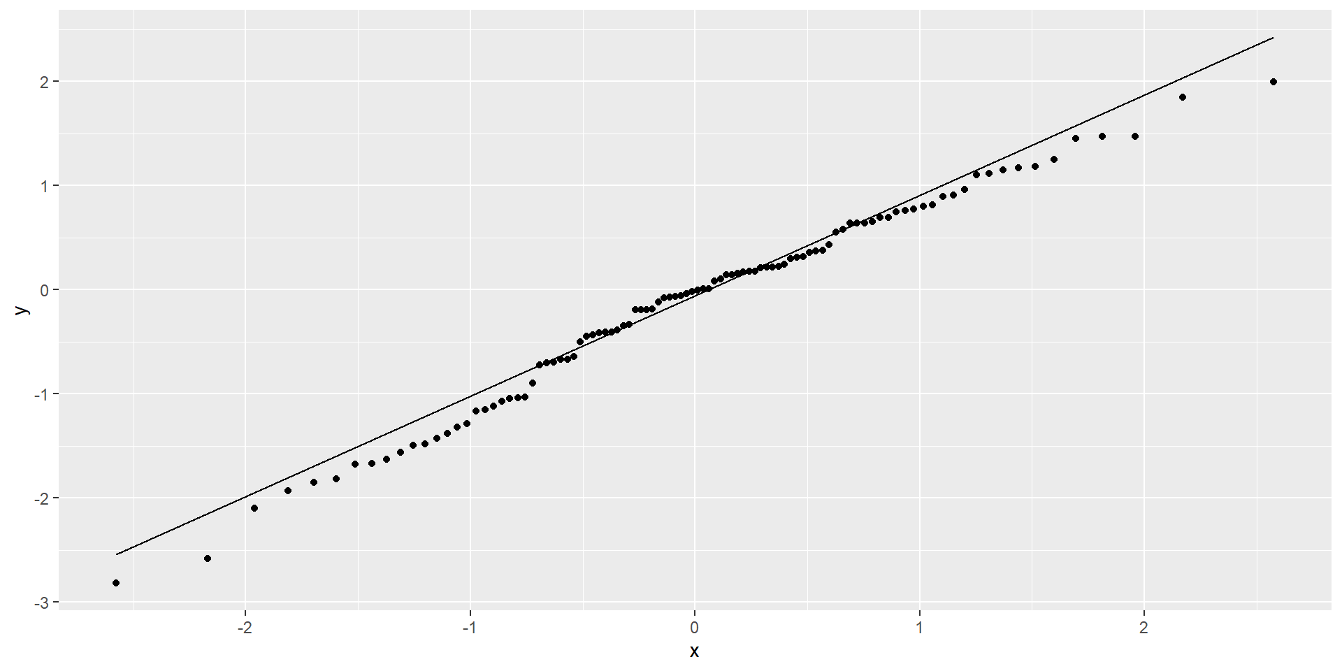
Diagnosing normality

• Assess visually with Q-Q plot
• Outliers (point with extreme residual) can result in violation of normality

Non-normal residuals

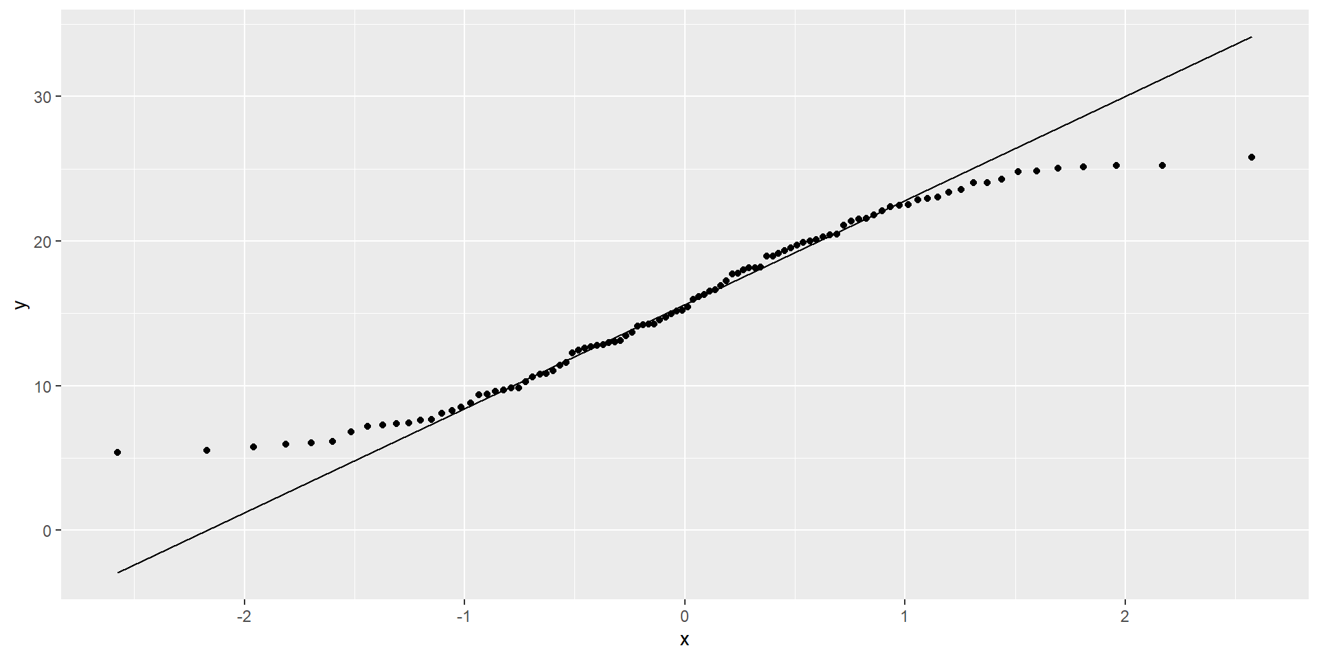
Normal residuals

When normality is violated

Implications:

• With no outliers and a large enough sample Central Limit Theorem corrects for lack of normality
• Can have biased predictions for \(Y\)

Remedies:

• Consider transformations of \(Y\)