Math 430: Lecture 5b
Linear Regression Model Evaluations
Professor Catalina Medina
How do we decide one model is better than another?
It depends on our purpose.
There are three values commonly used:
- Residual Standard Error (RSE)
- Root Mean Squared Deviation (RMSE)
- \(R^2\)
Residual Standard Error (RSE)
\[RSE = \hat{\sigma} = \sqrt{\frac{1}{n - 2} RSS} = \sqrt{\frac{1}{n - 2} \sum_{i = 1}^{n} (y_i - \hat{y}_i)^2}\]
- Measures lack of fit of the model to the data
- Measured in units of \(y\)
\(n - 2\) is required to make \(E[\hat{\sigma}^2] = \sigma^2\), but if often replaced by just \(n\) when the sole goal is prediction accuracy instead of inference
- using \(n\) instead of \(n - 2\) is called Root Mean Squared Error (RMSE)
What would you say is a “good” RSE/RMSE value? What would be a “bad” one?
- You can evaluate it relative to RSE/RMSE of another model (a model with different \(X\) for the same \(Y\))
- RMSE is “roughly” the average error, so you can think in context if the average error is acceptable or unacceptable
\(R^2\) statistic
\[R^2 = \frac{TSS - RSS}{TSS}\]
where \(TSS = \sum_{i = 1}^{n} (y_i - \bar{y})^2\).
- \(TSS\) measures amount of variability in \(Y\)
- \(RSS\) measures amount of variability in \(Y\) unexplained by model
- \(R^2\) measures percent of variability in \(Y\) explained by model
- \(TSS - RSS\) measures amount of variability explained by the model
\(R^2\) statistic
What \(R^2\) be for perfectly linear data?
What would \(R^2\) be for completely unlinear data?
In practice it is context specific for what constitutes a “reasonably good” \(R^2\)
- consider physics versus marketing
Correlation and the \(R^2\) statistic
\(Cor(X, Y) = \frac{\sum_{i = 1}^{n} (x_i - \bar{x})(y_i - \bar{y})}{\sqrt{\sum_{i = 1}^{n} (x_i - \bar{x})^2 }\sqrt{\sum_{i = 1}^{n} (y_i - \bar{y})^2}}\)
Correlation between \(X\) and \(Y\) is a measure of the linear relationship between \(X\) and \(Y\)
For simple linear regression \(R^2 = [Cor(X, Y)]^2\)
Cautions with \(R^2\)statistic
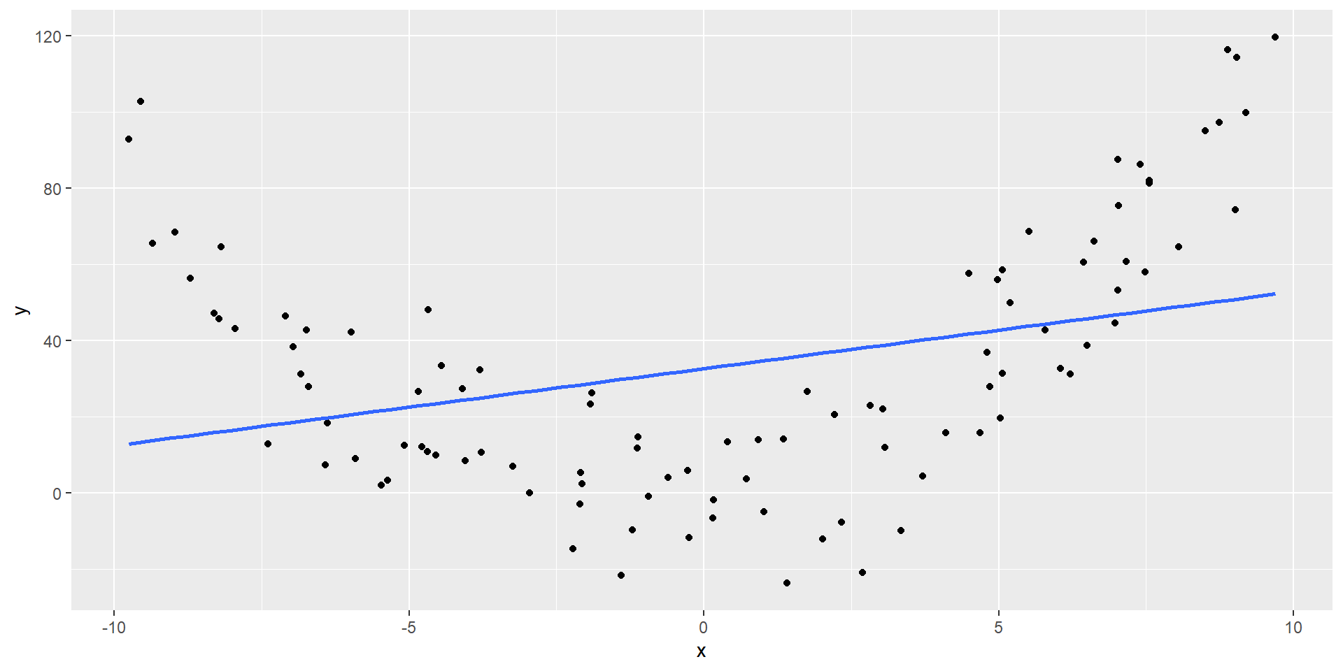
Low \(R^2\) does not mean no/(or weak) relationship, simply not a linear relationship
\(R^2\) = 0.11
Cautions with \(R^2\)statistic
High \(R^2\) does not mean a regression line fits the data well. Another function may describe it better
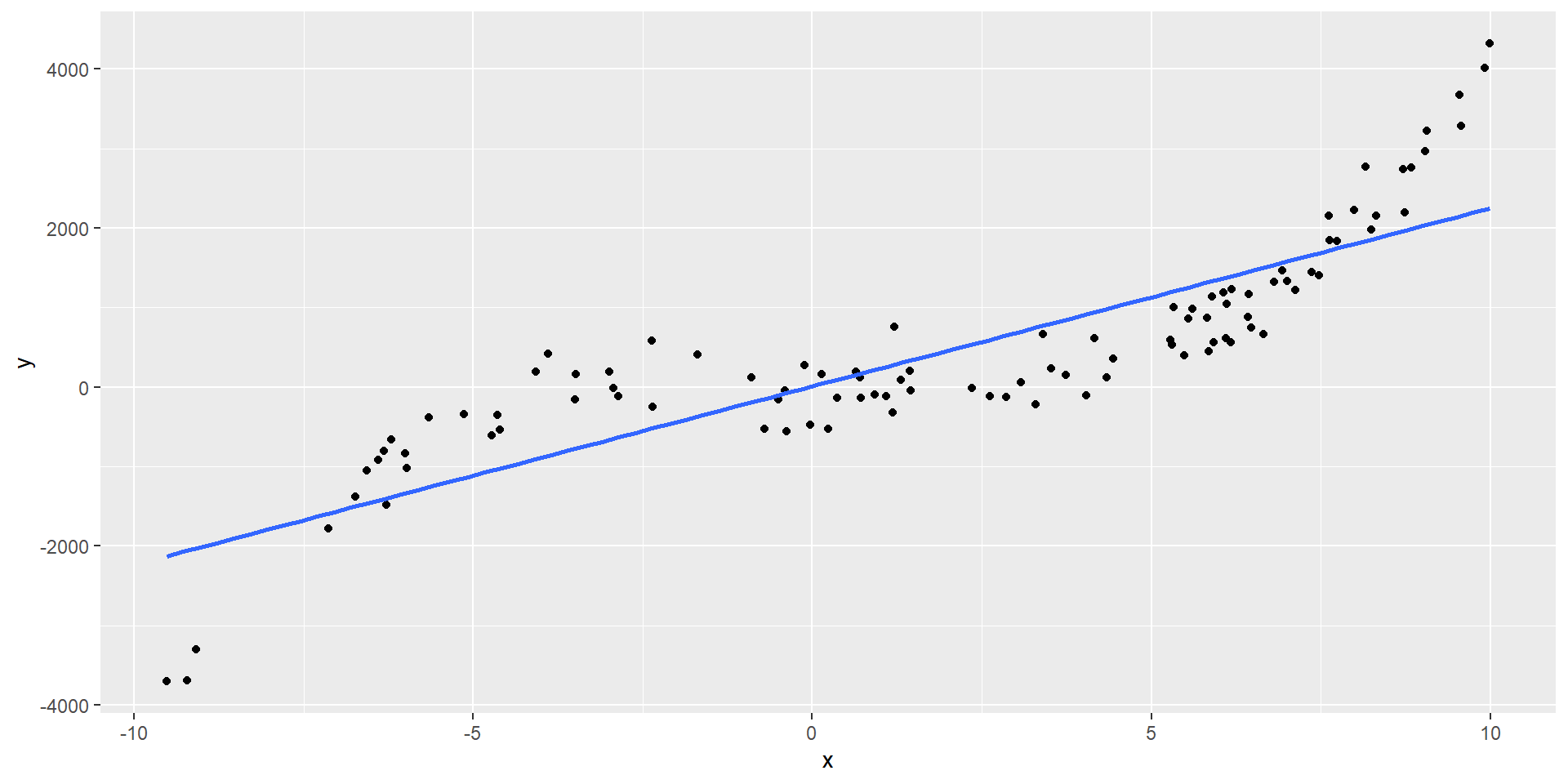
\(R^2\) = 0.74
Estimating the response
We know \(\hat{y}_i\) is our model’s point estimate for expectation of \(Y_i\)
What about an uncertainty estimate?
Confidence interval for average \(Y_i\)
Let \(\mu_Y = E[Y_i | X_i = x_h]\), the mean response when the explanatory variable value is \(x_h\). The confidence interval for \(\mu_y\) is:
\[\text{Point estimate} \pm t^* \times SE(\text{Point estiamte})\]
\[\hat{y}_h \pm t_{(1 - \alpha / 2, n - 2)} RSE\sqrt{ \left(\frac{1}{n} + \frac{(x_h - \bar{x})^2}{\sum_{i = 1}^{n} (x_i - \bar{x})^2}\right)}\]
- \(x_h\) must be within the range of the observed \(x_i\) values to avoid extrapolation, but need not be an observed \(x_i\)
Prediction interval for a new response
Let \(Y_{new}\) be the new response when the explanatory variable value is \(x_h\). The confidence interval for \(Y_{new}\) is:
\[\hat{y}_h \pm t_{(1 - \alpha / 2, n - 2)} RSE \sqrt{1 + \frac{1}{n} + \frac{(x_h - \bar{x})^2}{\sum_{i = 1}^{n} (x_i - \bar{x})^2}}\]
- \(x_h\) must be within the range of the observed \(x_i\) values to avoid extrapolation, but need not be an observed \(x_i\)
- How does this compare the the CI for average \(Y_i\)?
Example: Hospital infection risk
The hospital infection risk dataset consists of a sample of n = 58 hospitals in the east and north-central U.S. (Hospital Infection Data Region 1 and 2 data).
- The response variable is y = infection risk (percent of patients who get an infection).
- The explanatory variable is x = average length of stay (in days).
Example: Hospital infection risk data
hospital_infection <- read_tsv("https://online.stat.psu.edu/onlinecourses/sites/stat501/files/data/hospitalinfct_reg1and2.txt")

glimpse(hospital_infection)
Rows: 58
Columns: 12
$ ID <dbl> 5, 10, 11, 13, 18, 23, 27, 28, 29, 31, 33, 34, 36, 51, 55, …
$ Stay <dbl> 11.20, 8.84, 11.07, 12.78, 11.62, 9.78, 9.31, 8.19, 11.65, …
$ Age <dbl> 56.5, 56.3, 53.2, 56.8, 53.9, 52.3, 47.2, 52.1, 54.5, 49.9,…
$ InfctRsk <dbl> 5.7, 6.3, 4.9, 7.7, 6.4, 5.0, 4.5, 3.2, 4.4, 5.0, 5.3, 6.1,…
$ Culture <dbl> 34.5, 29.6, 28.5, 46.0, 25.5, 17.6, 30.2, 10.8, 18.6, 19.7,…
$ Xray <dbl> 88.9, 82.6, 122.0, 116.9, 99.2, 95.9, 101.3, 59.2, 96.1, 10…
$ Beds <dbl> 180, 85, 768, 322, 133, 270, 170, 176, 248, 318, 196, 312, …
$ MedSchool <dbl> 2, 2, 1, 1, 2, 1, 2, 2, 2, 2, 2, 2, 2, 2, 2, 2, 2, 2, 2, 1,…
$ Region <dbl> 1, 1, 1, 1, 1, 1, 1, 1, 1, 1, 1, 1, 1, 1, 1, 1, 1, 1, 1, 1,…
$ Census <dbl> 134, 59, 591, 252, 113, 240, 124, 156, 217, 270, 164, 258, …
$ Nurses <dbl> 151, 66, 656, 349, 101, 198, 173, 88, 189, 335, 165, 169, 1…
$ Facilities <dbl> 40.0, 40.0, 80.0, 57.1, 37.1, 57.1, 37.1, 37.1, 37.1, 57.1,…Example: Hospital infection risk model
Fitting the model
Call:
lm(formula = InfctRsk ~ Stay, data = hospital_infection)

Residuals:
    Min      1Q  Median      3Q     Max
-2.6145 -0.4660  0.1388  0.4970  2.4310

Coefficients:
            Estimate Std. Error t value Pr(>|t|)
(Intercept) -1.15982    0.95580  -1.213     0.23
Stay         0.56887    0.09416   6.041  1.3e-07 ***
---
Signif. codes:  0 '***' 0.001 '**' 0.01 '*' 0.05 '.' 0.1 ' ' 1

Residual standard error: 1.024 on 56 degrees of freedom
Multiple R-squared:  0.3946,    Adjusted R-squared:  0.3838
F-statistic:  36.5 on 1 and 56 DF,  p-value: 1.302e-07
Example: CI for Average risk of infection for average stay of 10 days?
new_hospital_data <- data.frame(Stay = 10)

predict(
  hospital_model,
  newdata = new_hospital_data,
  interval = "confidence",
  level = 0.95
)
fit lwr upr
1 4.528846 4.259205 4.798486We estimate the average risk of infection associated with a hospital with an average stay of 10 days to be 4.53. We estimate it to be between 4.26 and 4.8 with 95% confidence.
Example: Prediction interval for risk of infection for average stay of 10 days?
new_hospital_data <- data.frame(Stay = 10)

predict(
  hospital_model,
  newdata = new_hospital_data,
  interval = "prediction",
  level = 0.95
)
fit lwr upr
1 4.528846 2.45891 6.598781We estimate the risk of infection associated with a new hospital with an average stay of 10 days to be 4.53. We estimate it to be between 2.46 and 6.6 with 95% confidence.
Confidence bands
We can easily plot confidence bounds for average response - confidence intervals for average response for many \(x_i\)’s
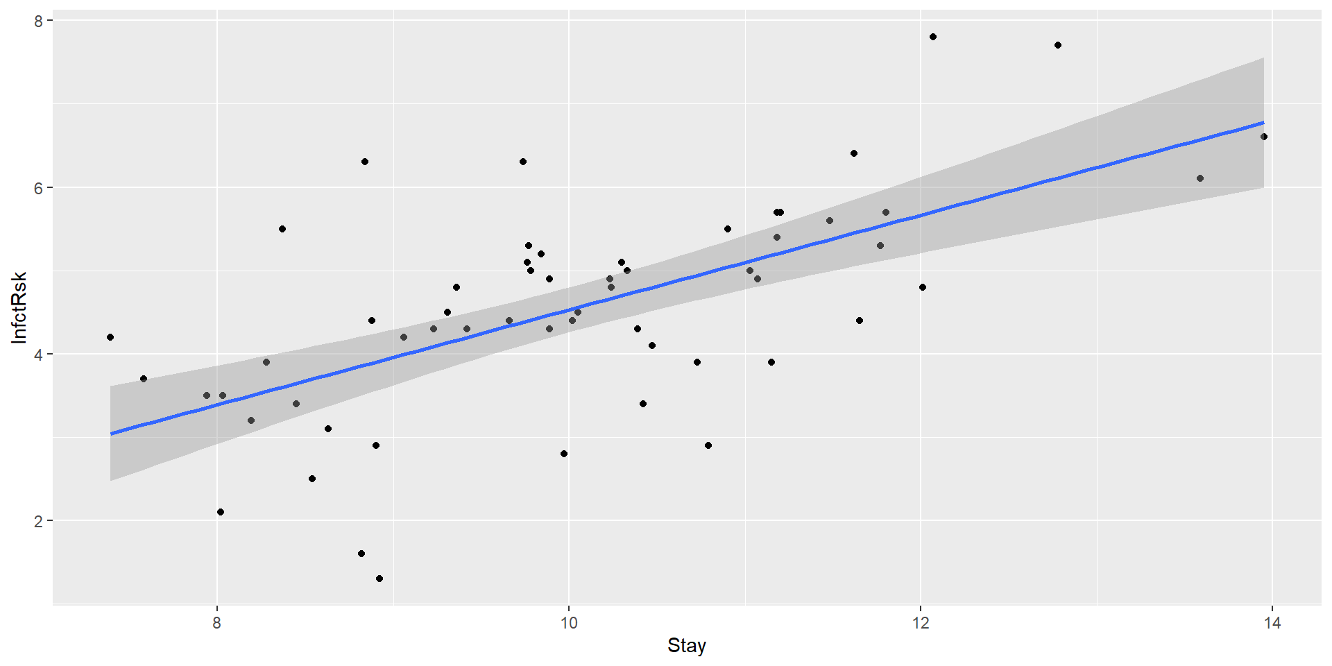
Confidence bands

The red line is our 95% confidence interval
Confidence bands
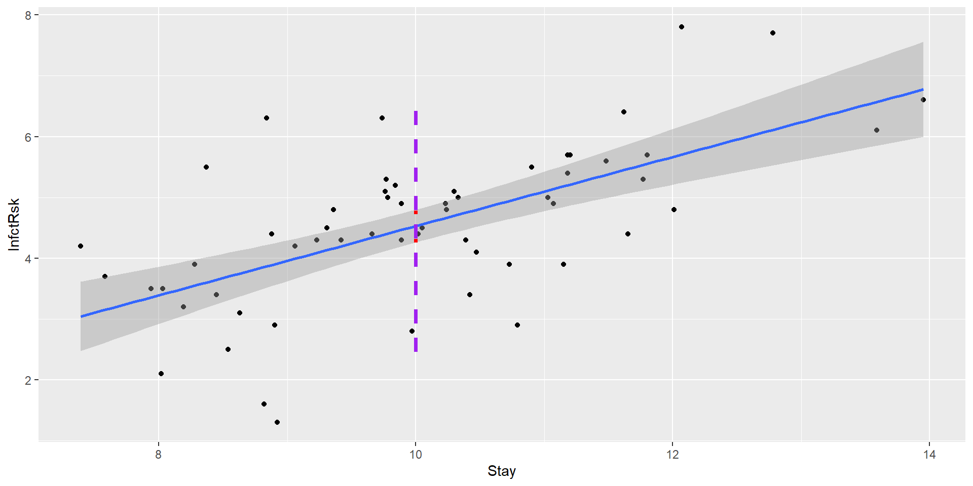
The purple line is the 95% prediction interval for a new hospital