Math 430: Lecture 6a
Multiple linear regression
Simple linear regression involves regressing \(Y\) on only one \(X\)
\[Y_i = \beta_0 + \beta_1 X_i + \epsilon_i,\]
with \(\epsilon_i \overset{iid}{\sim} N(0, \sigma^2)\).
Multiple linear regression involves regressing \(Y\) on multiple \(X\)’s
\[Y_i = \beta_0 + \beta_1 X_{1i} + \beta_2 X_{2i} + ... + \beta_p X_{pi} + \epsilon_i.\]
Why would we want multiple \(X\)’s?
Motivating example: Loan data
This dataset represents thousands of loans made through the Lending Club platform, which is a platform that allows individuals to lend to other individuals.
Motivating example: Loan data
You can type ? loans_full_schema into Console for the full data documentation.
Rows: 10,000
Columns: 57
$ emp_title                        <chr> "global config engineer ", "warehouse…
$ emp_length                       <dbl> 3, 10, 3, 1, 10, NA, 10, 10, 10, 3, 1…
$ state                            <fct> NJ, HI, WI, PA, CA, KY, MI, AZ, NV, I…
$ homeownership                    <fct> MORTGAGE, RENT, RENT, RENT, RENT, OWN…
$ annual_income                    <dbl> 90000, 40000, 40000, 30000, 35000, 34…
$ verified_income                  <fct> Verified, Not Verified, Source Verifi…
$ debt_to_income                   <dbl> 18.01, 5.04, 21.15, 10.16, 57.96, 6.4…
$ annual_income_joint              <dbl> NA, NA, NA, NA, 57000, NA, 155000, NA…
$ verification_income_joint        <fct> , , , , Verified, , Not Verified, , ,…
$ debt_to_income_joint             <dbl> NA, NA, NA, NA, 37.66, NA, 13.12, NA,…
$ delinq_2y                        <int> 0, 0, 0, 0, 0, 1, 0, 1, 1, 0, 0, 0, 0…
$ months_since_last_delinq         <int> 38, NA, 28, NA, NA, 3, NA, 19, 18, NA…
$ earliest_credit_line             <dbl> 2001, 1996, 2006, 2007, 2008, 1990, 2…
$ inquiries_last_12m               <int> 6, 1, 4, 0, 7, 6, 1, 1, 3, 0, 4, 4, 8…
$ total_credit_lines               <int> 28, 30, 31, 4, 22, 32, 12, 30, 35, 9,…
$ open_credit_lines                <int> 10, 14, 10, 4, 16, 12, 10, 15, 21, 6,…
$ total_credit_limit               <int> 70795, 28800, 24193, 25400, 69839, 42…
$ total_credit_utilized            <int> 38767, 4321, 16000, 4997, 52722, 3898…
$ num_collections_last_12m         <int> 0, 0, 0, 0, 0, 0, 0, 0, 0, 0, 0, 0, 0…
$ num_historical_failed_to_pay     <int> 0, 1, 0, 1, 0, 0, 0, 0, 0, 0, 1, 0, 0…
$ months_since_90d_late            <int> 38, NA, 28, NA, NA, 60, NA, 71, 18, N…
$ current_accounts_delinq          <int> 0, 0, 0, 0, 0, 0, 0, 0, 0, 0, 0, 0, 0…
$ total_collection_amount_ever     <int> 1250, 0, 432, 0, 0, 0, 0, 0, 0, 0, 0,…
$ current_installment_accounts     <int> 2, 0, 1, 1, 1, 0, 2, 2, 6, 1, 2, 1, 2…
$ accounts_opened_24m              <int> 5, 11, 13, 1, 6, 2, 1, 4, 10, 5, 6, 7…
$ months_since_last_credit_inquiry <int> 5, 8, 7, 15, 4, 5, 9, 7, 4, 17, 3, 4,…
$ num_satisfactory_accounts        <int> 10, 14, 10, 4, 16, 12, 10, 15, 21, 6,…
$ num_accounts_120d_past_due       <int> 0, 0, 0, 0, 0, 0, 0, NA, 0, 0, 0, 0, …
$ num_accounts_30d_past_due        <int> 0, 0, 0, 0, 0, 0, 0, 0, 0, 0, 0, 0, 0…
$ num_active_debit_accounts        <int> 2, 3, 3, 2, 10, 1, 3, 5, 11, 3, 2, 2,…
$ total_debit_limit                <int> 11100, 16500, 4300, 19400, 32700, 272…
$ num_total_cc_accounts            <int> 14, 24, 14, 3, 20, 27, 8, 16, 19, 7, …
$ num_open_cc_accounts             <int> 8, 14, 8, 3, 15, 12, 7, 12, 14, 5, 8,…
$ num_cc_carrying_balance          <int> 6, 4, 6, 2, 13, 5, 6, 10, 14, 3, 5, 3…
$ num_mort_accounts                <int> 1, 0, 0, 0, 0, 3, 2, 7, 2, 0, 2, 3, 3…
$ account_never_delinq_percent     <dbl> 92.9, 100.0, 93.5, 100.0, 100.0, 78.1…
$ tax_liens                        <int> 0, 0, 0, 1, 0, 0, 0, 0, 0, 0, 0, 0, 0…
$ public_record_bankrupt           <int> 0, 1, 0, 0, 0, 0, 0, 0, 0, 0, 1, 0, 0…
$ loan_purpose                     <fct> moving, debt_consolidation, other, de…
$ application_type                 <fct> individual, individual, individual, i…
$ loan_amount                      <int> 28000, 5000, 2000, 21600, 23000, 5000…
$ term                             <dbl> 60, 36, 36, 36, 36, 36, 60, 60, 36, 3…
$ interest_rate                    <dbl> 14.07, 12.61, 17.09, 6.72, 14.07, 6.7…
$ installment                      <dbl> 652.53, 167.54, 71.40, 664.19, 786.87…
$ grade                            <fct> C, C, D, A, C, A, C, B, C, A, C, B, C…
$ sub_grade                        <fct> C3, C1, D1, A3, C3, A3, C2, B5, C2, A…
$ issue_month                      <fct> Mar-2018, Feb-2018, Feb-2018, Jan-201…
$ loan_status                      <fct> Current, Current, Current, Current, C…
$ initial_listing_status           <fct> whole, whole, fractional, whole, whol…
$ disbursement_method              <fct> Cash, Cash, Cash, Cash, Cash, Cash, C…
$ balance                          <dbl> 27015.86, 4651.37, 1824.63, 18853.26,…
$ paid_total                       <dbl> 1999.330, 499.120, 281.800, 3312.890,…
$ paid_principal                   <dbl> 984.14, 348.63, 175.37, 2746.74, 1569…
$ paid_interest                    <dbl> 1015.19, 150.49, 106.43, 566.15, 754.…
$ paid_late_fees                   <dbl> 0, 0, 0, 0, 0, 0, 0, 0, 0, 0, 0, 0, 0…
$ bankruptcy                       <lgl> FALSE, TRUE, FALSE, FALSE, FALSE, FAL…
$ credit_util                      <dbl> 0.54759517, 0.15003472, 0.66134832, 0…
Motivating example: Loan data
interest_rateInterest rate on the loan, in an annual percentage.bankruptcyAn indicator variable for whether the borrower has a past bankruptcy in their record. This variable takes a value of1if the answer is yes and0if the answer is no.verified_incomeCategorical variable describing whether the borrower’s income source and amount have been verified, with levelsVerified(source and amount verified),Source Verified(source only verified), andNot Verified.
Categorical explanatory variables (aka Categorical “predictors” or Categorical “features”)
Regressing interest rate on bankruptcy
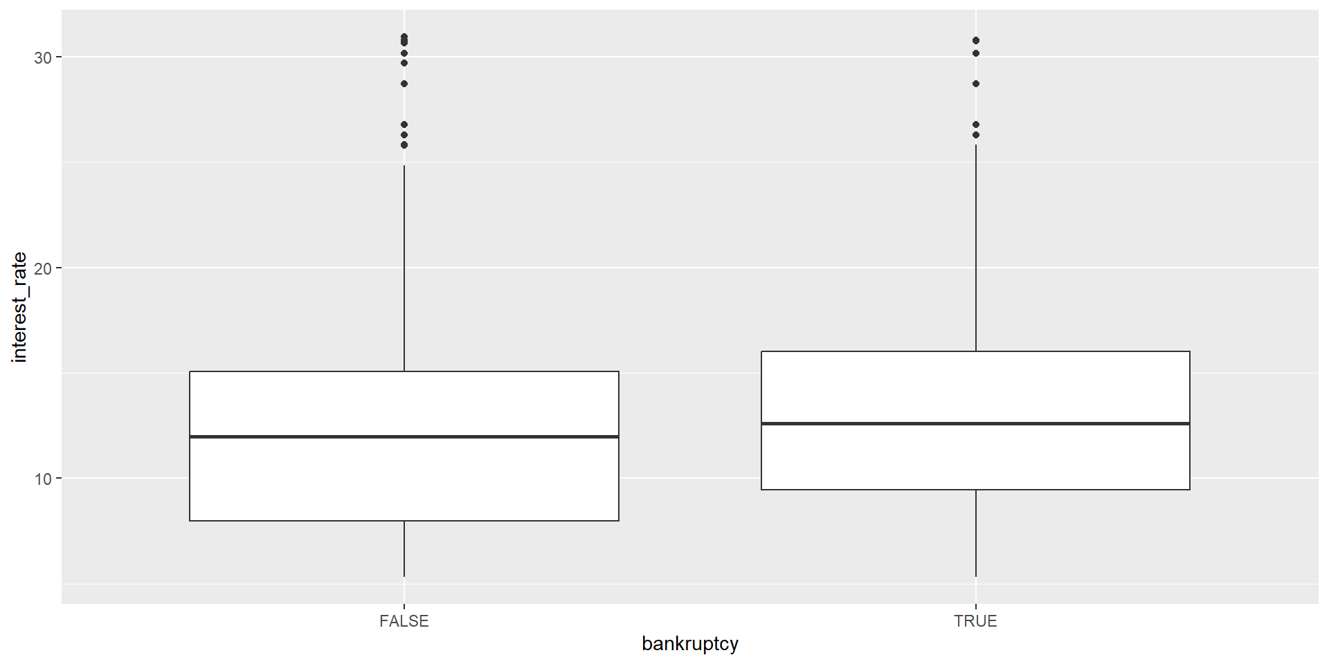
Regressing interest rate on bankruptcy
rate_on_bankruptcy_model <- lm(interest_rate ~ bankruptcy, data = loans)

summary(rate_on_bankruptcy_model)
Call:
lm(formula = interest_rate ~ bankruptcy, data = loans)

Residuals:
    Min      1Q  Median      3Q     Max
-7.7648 -3.6448 -0.4548  2.7120 18.6020

Coefficients:
               Estimate Std. Error t value Pr(>|t|)
(Intercept)     12.3380     0.0533 231.490  < 2e-16 ***
bankruptcyTRUE   0.7368     0.1529   4.819 1.47e-06 ***
---
Signif. codes:  0 '***' 0.001 '**' 0.01 '*' 0.05 '.' 0.1 ' ' 1

Residual standard error: 4.996 on 9998 degrees of freedom
Multiple R-squared:  0.002317,  Adjusted R-squared:  0.002217
F-statistic: 23.22 on 1 and 9998 DF,  p-value: 1.467e-06
How do we interpret the slope? What does it mean to be one unit more for X?
Regressing interest rate on bankruptcy: Fitted model
# A tibble: 2 × 5
  term           estimate std.error statistic    p.value
  <chr>             <dbl>     <dbl>     <dbl>      <dbl>
1 (Intercept)      12.3      0.0533    231.   0
2 bankruptcyTRUE    0.737    0.153       4.82 0.00000147
\(\hat{\text{Interest rate}}_i\) = 12.34
\(+\) 0.74 * \(I(\text{Bankruptcy}_i = \text{TRUE})\)
Regressing interest rate on bankruptcy: Interpreting coefficients
\(\hat{\text{Interest rate}}_i\) = 12.34
\(+\) 0.74 * \(I(\text{Bankruptcy}_i = \text{TRUE})\)
Definition:
\(I(\text{Bankruptcy}_i = \text{TRUE})\) is an indicator variable.
- It will be equal to 0 if the condition is not met
- It will be equal to 1 if the condition is met
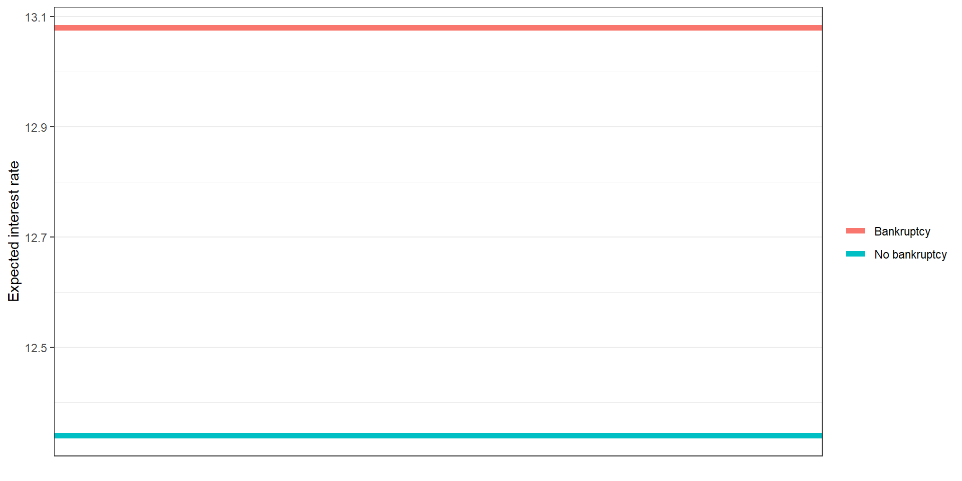
Regressing interest rate on bankruptcy: Interpreting coefficients
\(\hat{\text{Interest rate}}_i\) = 12.34
\(+\) 0.74 * \(I(\text{Bankruptcy}_i = \text{TRUE})\)
Expected interest rate for people with no bankruptcy on their record is 12.34.
Expected interest rate for people with at least one bankruptcy on their record is 13.08.
- The model predicts a 0.74% higher interest rate for borrowers with a bankruptcy on their record.
Regressing interest rate on bankruptcy
t-test versus regression
interest_rate_bankruptcy_false <- loans |>
  filter(bankruptcy == FALSE) |>
  pull(interest_rate)

interest_rate_bankruptcy_true <- loans |>
  filter(bankruptcy == TRUE) |>
  pull(interest_rate)

t.test(interest_rate_bankruptcy_false, interest_rate_bankruptcy_true)
    Welch Two Sample t-test

data:  interest_rate_bankruptcy_false and interest_rate_bankruptcy_true
t = -4.9599, df = 1598.6, p-value = 7.803e-07
alternative hypothesis: true difference in means is not equal to 0
95 percent confidence interval:
 -1.0281548 -0.4454164
sample estimates:
mean of x mean of y
 12.33800  13.07479
t-test versus regression
    Welch Two Sample t-test

data:  interest_rate_bankruptcy_false and interest_rate_bankruptcy_true
t = -4.9599, df = 1598.6, p-value = 7.803e-07
alternative hypothesis: true difference in means is not equal to 0
95 percent confidence interval:
 -1.0281548 -0.4454164
sample estimates:
mean of x mean of y
12.33800 13.07479 They are the same!
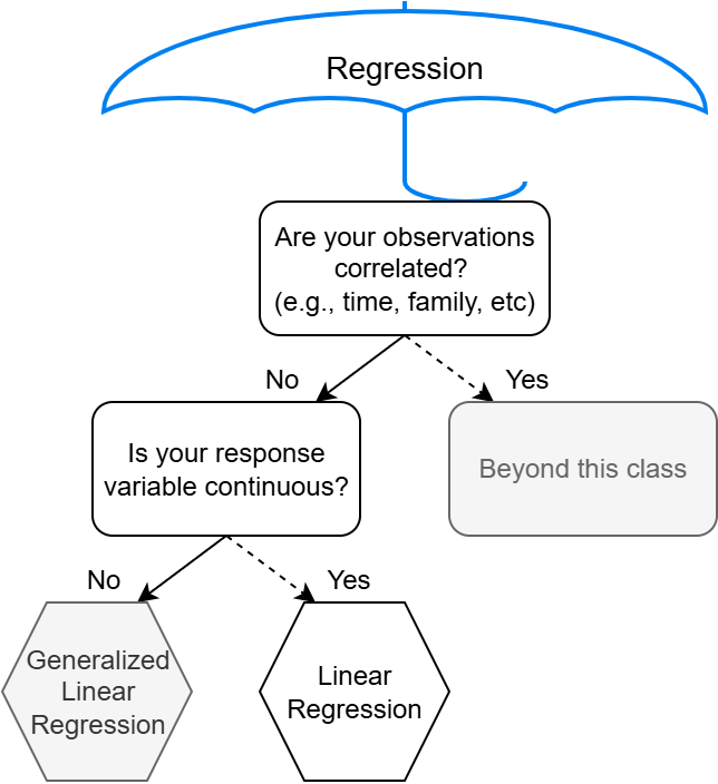
Regressing on categorical predictors
That was a continuous variable regression on a categorical variable with two levels (possibilities).
- Equivalent to a t-test.
- Our regression line is really two flat lines (means)
What if we regressed on a categorical variable with three or more levels (possibilities)?
Regressing interest rate on verified income
Notice that the verified_income variable is categorical with three levels
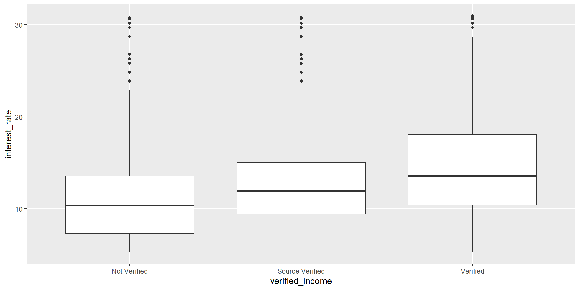
Regressing interest rate on verified income
rate_on_verification <- lm(interest_rate ~ verified_income, data = loans)

summary(rate_on_verification)
Call:
lm(formula = interest_rate ~ verified_income, data = loans)

Residuals:
    Min      1Q  Median      3Q     Max
-9.0437 -3.7495 -0.6795  2.5345 19.6905

Coefficients:
                               Estimate Std. Error t value Pr(>|t|)
(Intercept)                    11.09946    0.08091  137.18   <2e-16 ***
verified_incomeSource Verified  1.41602    0.11074   12.79   <2e-16 ***
verified_incomeVerified         3.25429    0.12970   25.09   <2e-16 ***
---
Signif. codes:  0 '***' 0.001 '**' 0.01 '*' 0.05 '.' 0.1 ' ' 1

Residual standard error: 4.851 on 9997 degrees of freedom
Multiple R-squared:  0.05945,   Adjusted R-squared:  0.05926
F-statistic: 315.9 on 2 and 9997 DF,  p-value: < 2.2e-16
Fitted interest rate model: Fitted model
# A tibble: 3 × 5
  term                           estimate std.error statistic   p.value
  <chr>                             <dbl>     <dbl>     <dbl>     <dbl>
1 (Intercept)                       11.1     0.0809     137.  0
2 verified_incomeSource Verified     1.42    0.111       12.8 3.79e- 37
3 verified_incomeVerified            3.25    0.130       25.1 8.61e-135
Our model appears to be
\(\hat{\text{Interest rate}}_i\) =11.1
+ 1.42 \(I(\text{verified_income}_i = \text{Source Verified})\)
+ 3.25 \(I(\text{verified_income}_i = \text{Verified}).\)
Is anything missing?
Categorical predictors
When fitting a regression model with a categorical variable that has \(k\) levels where \(k \geq 2\), software will provide a coefficient for \(k-1\) of those levels.
- For the last level that does not receive a coefficient, this is the reference level, and the coefficients listed for the other levels are all considered relative to this reference level.
Expected difference in interest ratec
\(\hat{\text{Interest rate}}_i\) =11.1
+ 1.42 \(I(\text{verified_income}_i = \text{Source Verified})\)
+ 3.25 \(I(\text{verified_income}_i = \text{Verified}).\)
- We expect a 1.42% higher interest rate for people source only verified relative to unverified people.
- We expect a 3.25% higher interest rate for people source and amount verified relative to unverified people.
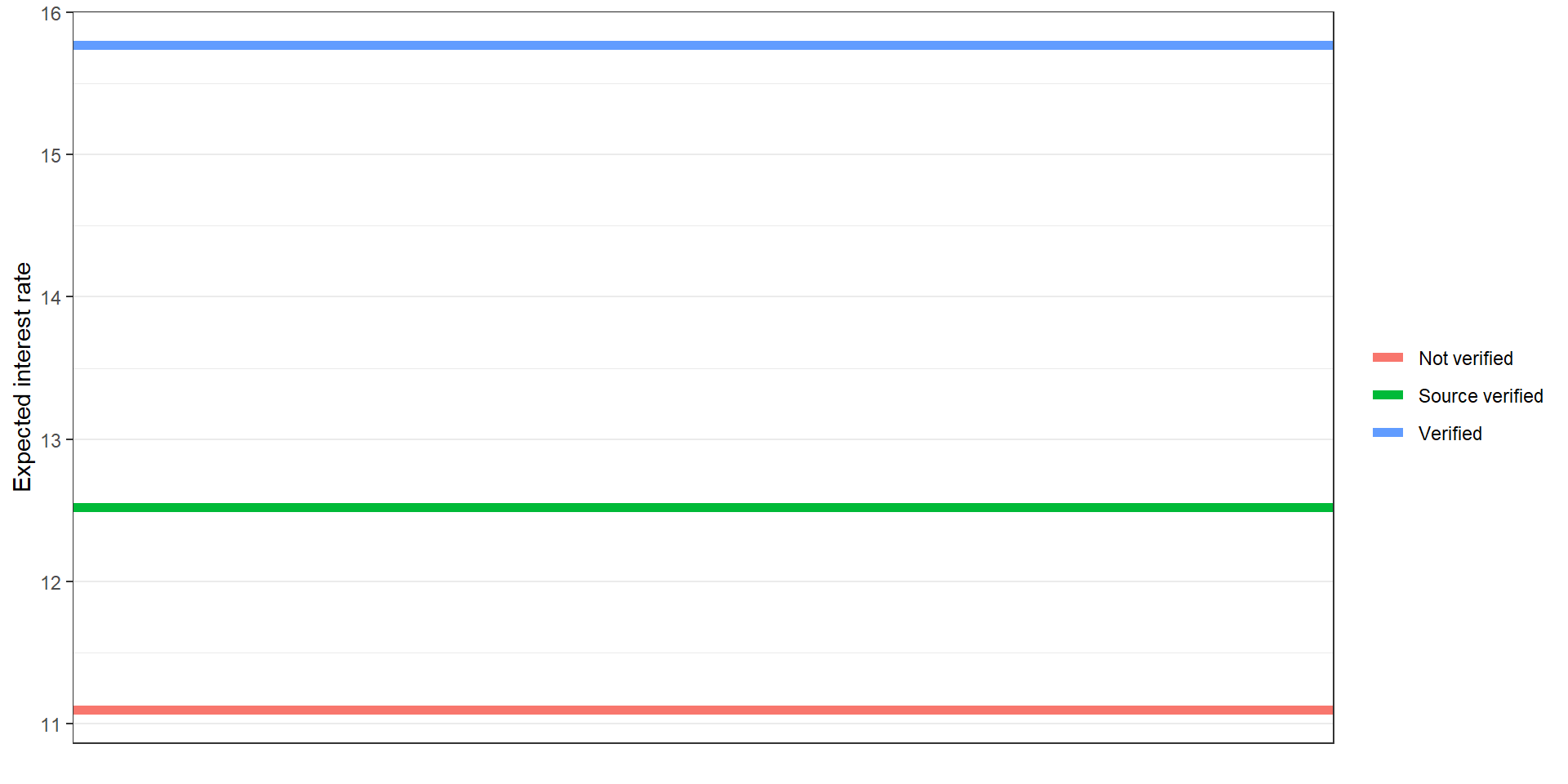
Expected interest rate
\(\hat{\text{Interest rate}}_i\) =11.1
+ 1.42 \(I(\text{verified_income}_i = \text{Source Verified})\)
+ 3.25 \(I(\text{verified_income}_i = \text{Verified}).\)
Expected interest rate for people not verified is 11.1.
Expected interest rate for people source only verified is 12.52.
Expected interest rate for people source and amount verified is 15.77.
Expected interest rate
Converting categorical variables to numeric in regression
Why shouldn’t we just convert the verified_income variable to a numeric?
Converting categorical variables to numeric in regression
rate_on_ver_num_model <- lm(interest_rate ~ verified_income_numeric, data = loans)

summary(rate_on_ver_num_model)
Call:
lm(formula = interest_rate ~ verified_income_numeric, data = loans)

Residuals:
    Min      1Q  Median      3Q     Max
-8.9344 -3.6798 -0.6544  2.5602 19.7602

Coefficients:
                        Estimate Std. Error t value Pr(>|t|)
(Intercept)             11.02980    0.07395  149.15   <2e-16 ***
verified_income_numeric  1.60731    0.06418   25.04   <2e-16 ***
---
Signif. codes:  0 '***' 0.001 '**' 0.01 '*' 0.05 '.' 0.1 ' ' 1

Residual standard error: 4.852 on 9998 degrees of freedom
Multiple R-squared:  0.05903,   Adjusted R-squared:  0.05893
F-statistic: 627.2 on 1 and 9998 DF,  p-value: < 2.2e-16
Converting categorical variables to numeric in regression
\(\hat{\beta_1} = 1.61\)
By converting we are implicitly assuming that there is a one unit difference between each of the levels:
- Not verified -> Source only verified
- Source only verified -> Source and amount verified
This may not be the case, maybe “Source only verified” and “Source and amount verified” are more similar than “Not verified”
Not good practice!
Multiple predictors of different variable types
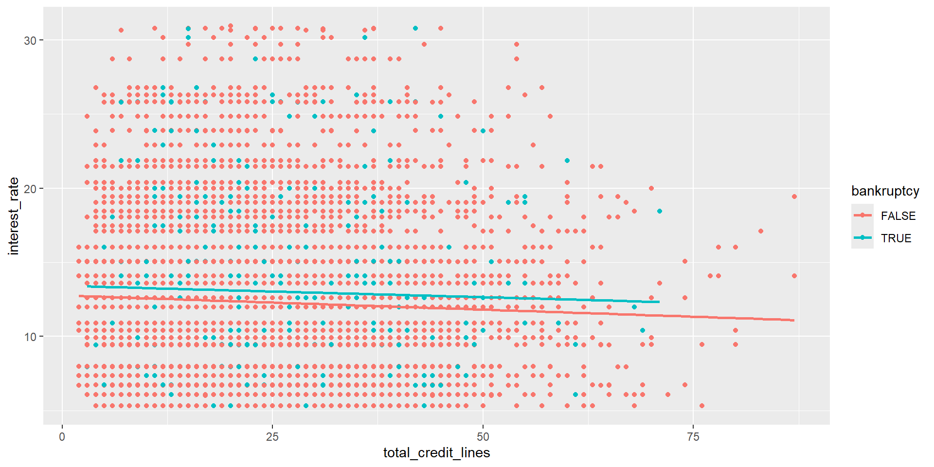
Regressing interest rate on bankruptcy and credit lines
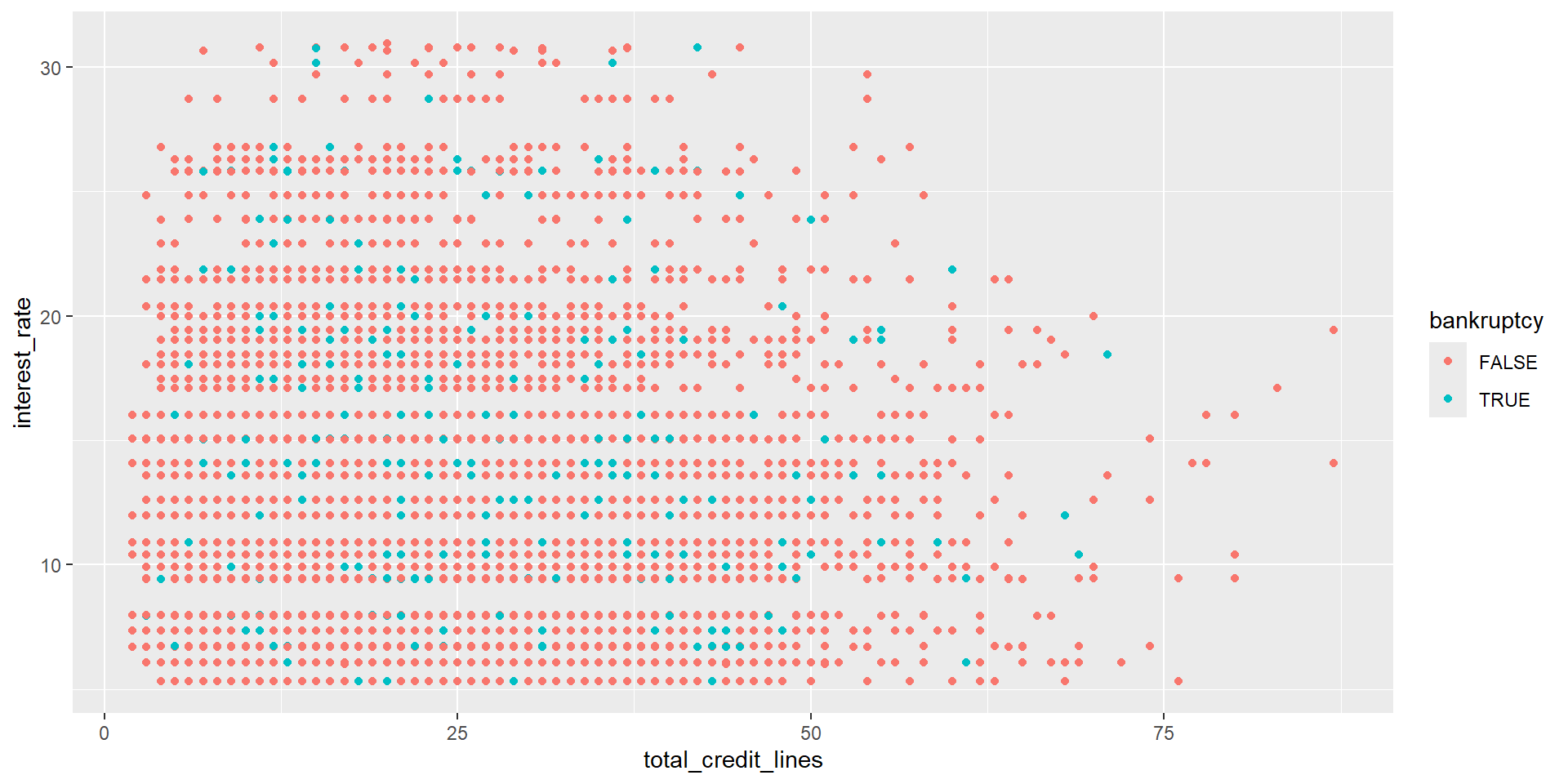
Regressing interest rate on bankruptcy and credit lines
rate_on_bank_and_credit_model <- lm(interest_rate ~ bankruptcy + total_credit_lines, data = loans)

summary(rate_on_bank_and_credit_model)
Call:
lm(formula = interest_rate ~ bankruptcy + total_credit_lines,
    data = loans)

Residuals:
    Min      1Q  Median      3Q     Max
-7.9651 -3.7041 -0.6226  2.7263 18.8697

Coefficients:
                    Estimate Std. Error t value Pr(>|t|)
(Intercept)        12.762332   0.109102 116.976  < 2e-16 ***
bankruptcyTRUE      0.737299   0.152762   4.826 1.41e-06 ***
total_credit_lines -0.018712   0.004199  -4.456 8.44e-06 ***
---
Signif. codes:  0 '***' 0.001 '**' 0.01 '*' 0.05 '.' 0.1 ' ' 1

Residual standard error: 4.991 on 9997 degrees of freedom
Multiple R-squared:  0.004295,  Adjusted R-squared:  0.004095
F-statistic: 21.56 on 2 and 9997 DF,  p-value: 4.54e-10
Regressing interest rate on bankruptcy and credit lines
# A tibble: 3 × 5
  term               estimate std.error statistic    p.value
  <chr>                 <dbl>     <dbl>     <dbl>      <dbl>
1 (Intercept)         12.8      0.109      117.   0
2 bankruptcyTRUE       0.737    0.153        4.83 0.00000141
3 total_credit_lines  -0.0187   0.00420     -4.46 0.00000844
\(\hat{\text{Interest rate}}_i\) = 12.76
\(+\) 0.74 \(I(\text{Banruptcy_i = TRUE})\)
\(+\) -0.02 \(\text{Number credit lines}_i\)
Interpreting estimates
\(\hat{\text{Interest rate}}_i\) = 12.76
\(+\) 0.74 \(I(\text{Banruptcy_i = TRUE})\)
\(+\) -0.02 \(\text{Number credit lines}_i\)
- We expect an interest rate of 12.76 for people with no bankruptcy and no lines of credit.
Interpreting estimates
\(\hat{\text{Interest rate}}_i\) = 12.76
\(+\) 0.74 \(I(\text{Banruptcy_i = TRUE})\)
\(+\) -0.02 \(\text{Number credit lines}_i\)
We interpret a slope with all other variables fixed:
- We expect a 0.74% higher interest rate for borrowers with a bankruptcy on their record, for people with similar number of lines of credit.
- We expect a 0.02% decrease in interest rate associated with having one additional line of credit, for people with the same bankruptcy history.
Regressing interest rate on bankruptcy and credit lines