Math 430: Lecture 6b

Multiple linear regression

Professor Catalina Medina

Some important questions

When we perform multiple linear regression, we usually are interested in answering a few important questions.

Is at least one of the predictors \(X_1, X_2,...,X_p\) useful in predicting the response?
Do all the predictors help to explain \(Y\) , or is only a subset of the predictors useful?
How well does the model fit the data?
Given a set of predictor values, what response value should we predict, and how accurate is our prediction?

Q1: Is There a Linear Relationship Between the Response and Predictors?

Q1 with simple linear regression

\[Y_i = \beta_0 + \beta_1 X_i + \epsilon_i\]

Hypothesis test for \(\beta_1\)!

\(H_0: \beta_1 = 0\)
\(H_A: \beta_1 \neq 0\)
Compute p-value.

What is the definition of p-value?

Judge if you (1) found evidence against the null hypothesis (in support of the alternative) or (2) failed to find evidence against the null hypothesis (failed to find evidence to support the alternative)

Q1 with multiple linear regression

\[Y_i = \beta_0 + \beta_1 X_{1i} + \beta_2 X_{2i} + ... + \beta_p X_{p,i} + \epsilon_i\]

Hypothesis test for all \(\beta_j\)’s!

\(H_0: \beta_1 = \beta_2 = \dots = \beta_p = 0\)
\(H_A\): At least one \(\beta_j\) is non-zero
Compute p-value.
Judge if you (1) found evidence against the null hypothesis (in support of the alternative) or (2) failed to find evidence against the null hypothesis (failed to find evidence to support the alternative)

F-statistic

\(H_0: \beta_1 = \beta_2 = \dots = \beta_p = 0\)
\(H_A\): At least one \(\beta_j\) is non-zero

Our test test statistic for the hypothesis test is: \[F = \frac{(TSS - RSS) / p}{RSS / (n - p -1)}\]

TSS = …
RSS = …
n = …
p = …

F-statistic (in practice)

The dataset contains data on test performance, school characteristics and student demographic backgrounds for school districts in California in 1999.

ca_schools_og <- read_csv(
  "http://csuci-math430.github.io/lectures/data/CASchools.csv",
  show_col_types = FALSE
)

ca_schools <- ca_schools_og |> 
  mutate(student_teacher_ratio = students / teachers) |> 
  mutate(student_computer_ratio = case_when(
    computer != 0 ~ students / computer,
    computer == 0 ~ 0
  )) |> 
  mutate(ave_score = (read + math) / 2)

California Schools data

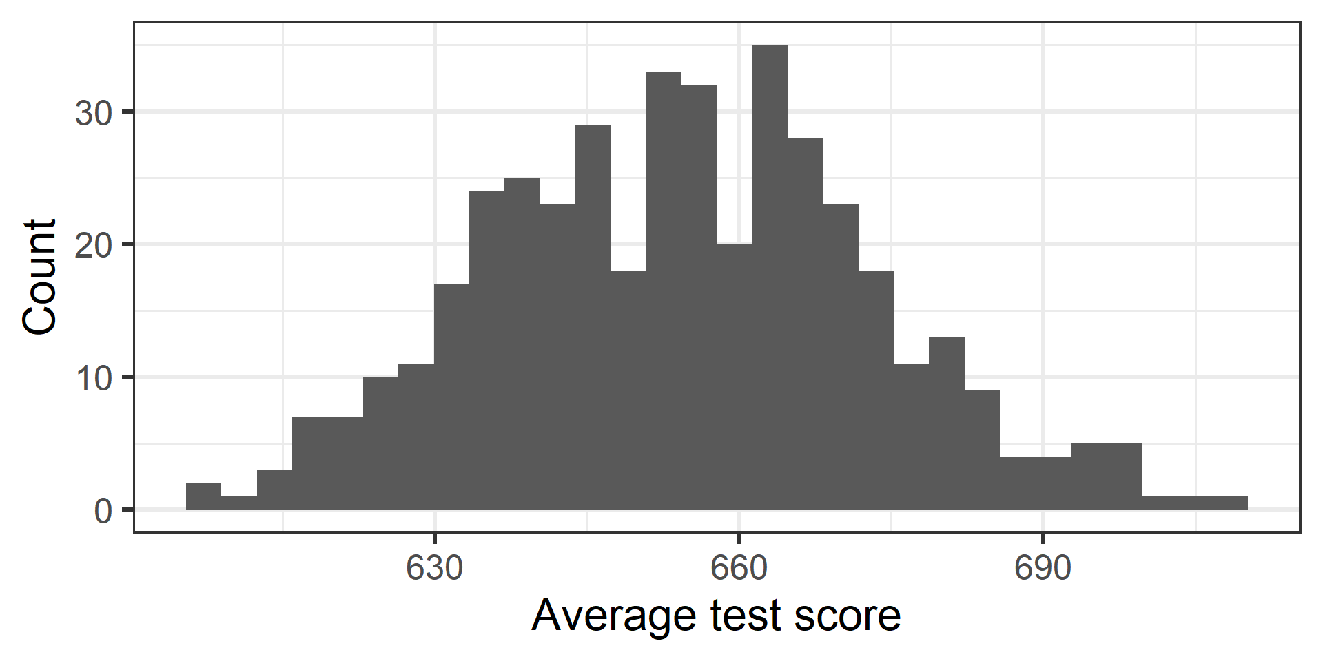
California Schools data

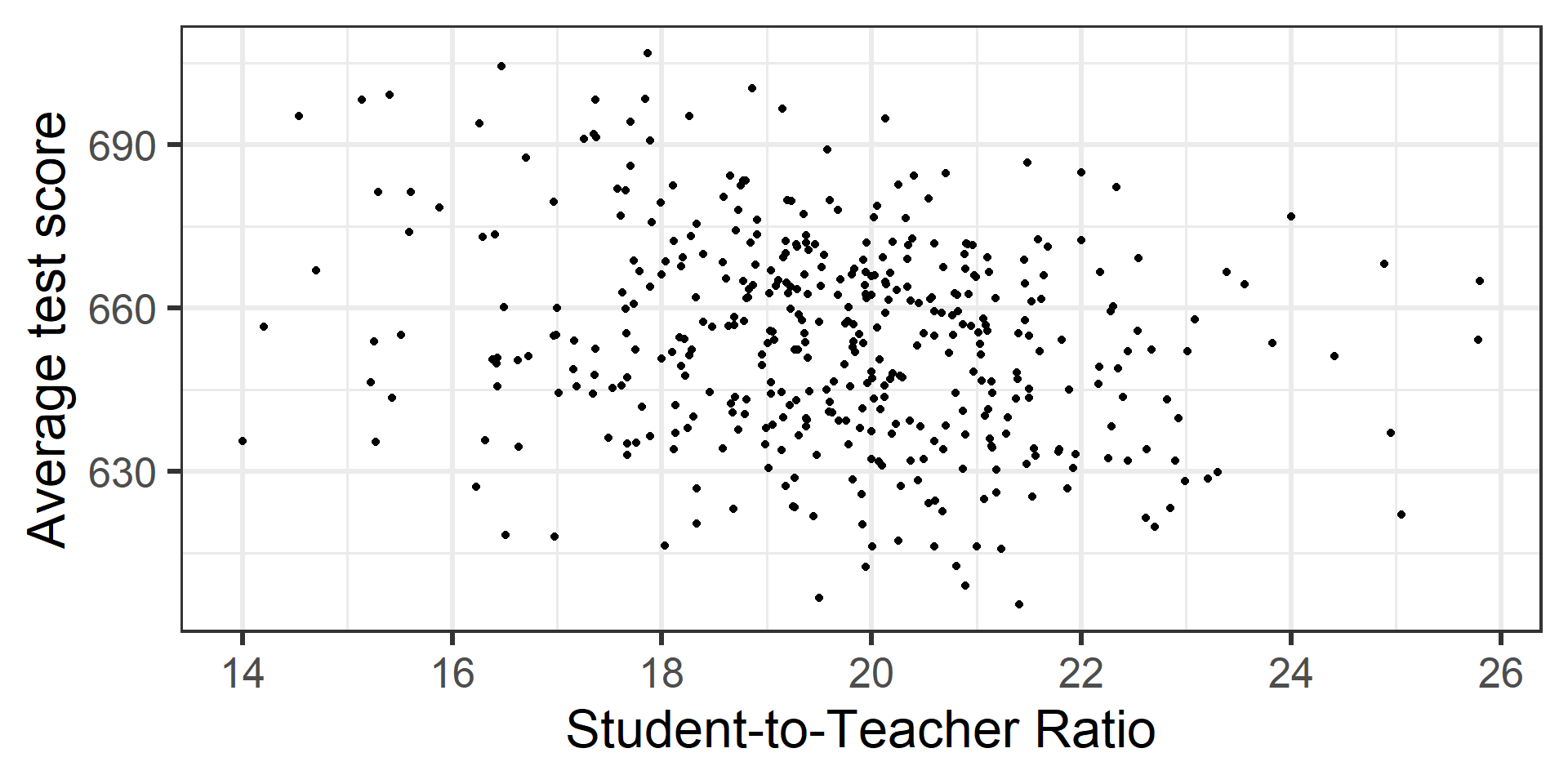
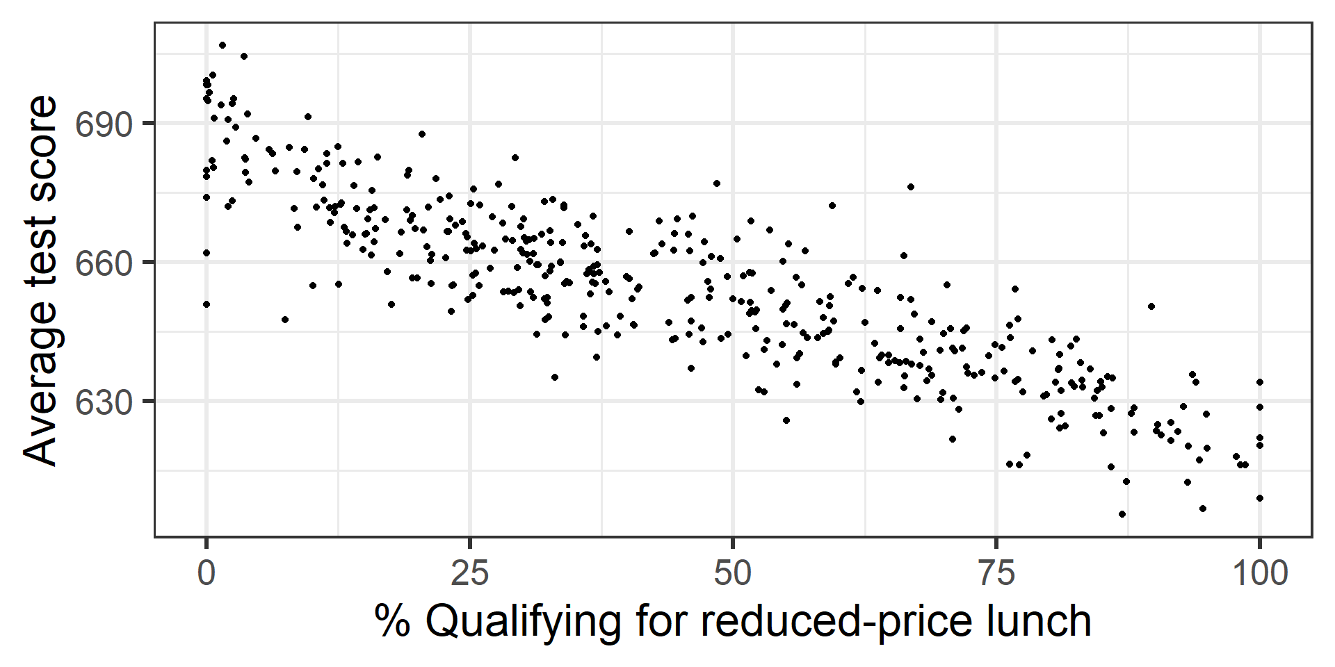
We are going to regress average test score on student-to-teacher ratio, student-to-computer ratio, and percent qualifying for reduced-price lunch.

\[\begin{equation*} \begin{split} &\text{Score}_i = \beta_0 \\ &+ \beta_1 \text{Student-Teacher Ratio}_i\\ &+ \beta_2 \text{Student-Computer Ratio}_i \\ &+ \beta_3 \text{\% Reduced Price Lunch}_i\\ &+ \epsilon_i \end{split} \end{equation*}\]

F-statistic (in practice)

score_model1 <- lm(
  ave_score ~ student_teacher_ratio + student_computer_ratio + lunch, 
  data = ca_schools
)

summary(score_model1)


Call:
lm(formula = ave_score ~ student_teacher_ratio + student_computer_ratio + 
    lunch, data = ca_schools)

Residuals:
    Min      1Q  Median      3Q     Max 
-34.117  -5.323  -0.262   5.674  33.241 

Coefficients:
                        Estimate Std. Error t value Pr(>|t|)    
(Intercept)            703.03249    4.66790 150.610  < 2e-16 ***
student_teacher_ratio   -1.04075    0.24047  -4.328 1.89e-05 ***
student_computer_ratio  -0.21938    0.08388  -2.615  0.00924 ** 
lunch                   -0.59305    0.01684 -35.208  < 2e-16 ***
---
Signif. codes:  0 '***' 0.001 '**' 0.01 '*' 0.05 '.' 0.1 ' ' 1

Residual standard error: 9.158 on 416 degrees of freedom
Multiple R-squared:  0.7706,    Adjusted R-squared:  0.769 
F-statistic: 465.9 on 3 and 416 DF,  p-value: < 2.2e-16

F-statistic (in practice)

What if you want to extract the F-statistic or its p-value?

library(broom)

glance(score_model1)

# A tibble: 1 × 12
  r.squared adj.r.squared sigma statistic   p.value    df logLik   AIC   BIC
      <dbl>         <dbl> <dbl>     <dbl>     <dbl> <dbl>  <dbl> <dbl> <dbl>
1     0.771         0.769  9.16      466. 1.42e-132     3 -1524. 3058. 3078.
# ℹ 3 more variables: deviance <dbl>, df.residual <int>, nobs <int>

glance(score_model1) |> 
  pull(statistic)

   value 
465.8531

glance(score_model1) |> 
  pull(p.value)

        value 
1.421696e-132

Notice we could also extract \(R^2\) and \(RSE = \hat{\sigma}\)!

F-statistic (in practice)

\(H_0: \beta_1 = \beta_2 = \dots = \beta_p = 0\)
\(H_A\): At least one \(\beta_j\) is non-zero

Statistics conclusion: Our p-value is 1.4216963^{-132}. Therefore there is very strong evidence against \(H_0\) in support of \(H_A\).

Conclusion in context: We found very strong evidence (p-value = 1.4216963^{-132}) that at least one of student-teacher ratio, student-computer ratio, or % reduced lunch is linearly related to score.

Partial F-test for nested models

From the plots it was pretty clear lunch is linearly related to score. What if we only wanted to do a test to see if student-teacher ratio and or student-computer ratio is linearly related to score?

We can do a partial F-test for nested models!

\(H_0: \beta_1 = \beta_2 = 0\)
\(H_A:\) At least one of \(\beta_1\) or \(\beta_2\) are nonzero.

F-test with subset of coefficients

score_model1 <- lm(
  ave_score ~ student_teacher_ratio + student_computer_ratio + lunch,
  data = ca_schools
)

score_model2 <- lm(
  ave_score ~ lunch,
  data = ca_schools
)

anova(score_model2, score_model1)

Analysis of Variance Table

Model 1: ave_score ~ lunch
Model 2: ave_score ~ student_teacher_ratio + student_computer_ratio + 
    lunch
  Res.Df   RSS Df Sum of Sq      F    Pr(>F)    
1    418 37303                                  
2    416 34891  2    2411.2 14.374 9.196e-07 ***
---
Signif. codes:  0 '***' 0.001 '**' 0.01 '*' 0.05 '.' 0.1 ' ' 1

F-test with subset of coefficients

partial_f_test <- anova(score_model2, score_model1)
partial_f_test_p_value <- partial_f_test$`Pr(>F)`[2]

Statistics conclusion: Our p-value is 9.1955202^{-7}. Therefore there is very strong evidence against \(H_0\) in support of \(H_A\).

Conclusion in context: We found very strong evidence (p-value = 9.1955202^{-7}) that at least one of student-teacher ratio or student-computer ratio is linearly related to score, in addition to lunch.

Why F-test instead of regular t-test??

tidy(score_model1)

# A tibble: 4 × 5
  term                   estimate std.error statistic   p.value
  <chr>                     <dbl>     <dbl>     <dbl>     <dbl>
1 (Intercept)             703.       4.67      151.   0        
2 student_teacher_ratio    -1.04     0.240      -4.33 1.89e-  5
3 student_computer_ratio   -0.219    0.0839     -2.62 9.24e-  3
4 lunch                    -0.593    0.0168    -35.2  7.65e-127

tidy(score_model2)

# A tibble: 2 × 5
  term        estimate std.error statistic   p.value
  <chr>          <dbl>     <dbl>     <dbl>     <dbl>
1 (Intercept)  681.       0.889      766.  0        
2 lunch         -0.610    0.0170     -35.9 1.19e-129

For instance, consider an example in which \(p = 100\) and \(H_0 : \beta_1 = \beta_2 =··· = \beta_p = 0\) is true, so no variable is truly associated with the response.

Imagine we collected a bunch of samples
With a boundary (significance level) of 0.05, we will see approximately 5% of p-values for each predictor below 0.05 by chance
Our significance level is actually the type I error rate, the probability of incorrectly rejecting a true null hypothesis (“false positive”)
An F-statistic adjusts for \(p\)

Q2: Do all the predictors help to explain \(Y\), or is only a subset of the predictors useful?

Statistical Inference

If you are doing statistical inference you need to be conscious not to increase your type I error rate (e.g. Pharmaceutical setting testing if Drug A lowers cholesterol relative to Drug B).

Therefore you should consider ahead of time what predictors should be included based on the scientific peer-reviewed literature
You should not fit a bunch of models, see what “fits best”, then do a hypothesis test (“p-hacking”)
After you answer your question of interest you can then do exploratory analyses

Prediction

Fit a bunch of models and see what “fits best”

We will cover this in week 12

Q3 How well does the model fit the data?

Metrics we already know

RSE for multiple linear regression

\[RSE = \sqrt{\frac{RSS}{n - p -1}}\]

Reduces to \(RSE = \sqrt{\frac{RSS}{n - 2}}\) for simple linear regression

\(R^2\)

\[R^2 = \frac{TSS - RSS}{TSS} = 1 - \frac{RSS}{TSS}\]

\(R^2\) will always increase as \(p\) increases

\[\text{Adjusted }R^2 = 1 - \frac{RSS (n - 1)}{TSS (n - p - 1)}\]

No longer has the same interpretation as \(R^2\)

Q4 Given a set of predictor values, what response value should we predict, and how accurate is our prediction?

Same as with simple linear regression!

We can compute a prediction by plugging in values for all of our \(X_j\)’s into our fitted model
We can compute a prediction interval

What do we predict the average test score will be for a school with a student-teacher ratio of 22, student-computer ratio of 10, and 50% qualifying for reduced-price lunch?

my_new_data <- data.frame(
  student_teacher_ratio = 22,
  student_computer_ratio = 10,
  lunch = 50
)

predict(score_model1, newdata = my_new_data, interval = "prediction")

       fit      lwr      upr
1 648.2898 630.2328 666.3468

my_pred <- predict(score_model1, newdata = my_new_data, interval = "prediction")

We predict their average test score to be 648.29, between 630.23 and 666.35 with 95% confidence.