Math 430: Lecture 8a

Logistic regression

Professor Catalina Medina

Examples of Outcome Variables

Specify variable type (think about the possible values)

  • Temperature

  • Presence of Alzheimer’s

  • Rent

  • Computer operating system

  • Daily number of customers

  • Income class

Which could we model with linear regression?

Identify the response variable type:

  • A car insurance company is trying to predict if an applicant will have a car crash in the next 5 years, based on their income.

Can we model using linear regression anyways?

Let’s simulated data…

What does it mean to fit a line to this data?

We don’t get an error, but …

Linear regression assumes \[Y_i = \beta_0 + \beta_1 X_{1, i} + ... + \beta_p X_{p, i} + \epsilon_i \text{ and } \epsilon_i\sim N(0, \sigma^2)\]

so

\[E[Y_i | X_{1, i}, ..., X_{p, i}] = \beta_0 + \beta_1 X_{1, i} + ... + \beta_p X_{p, i}\]

What is the expectation of a binary variable?

What is our expecation for people with an income of $45,000?

crash_model <- lm(car_crash ~ income, data = sim_crash_data)

new_data <- data.frame(income = 45)

predict(crash_model, newdata = new_data)
        1 
0.4151667 

What is our expecation for people with an income of $90,000?

crash_model <- lm(car_crash ~ income, data = sim_crash_data)

new_data <- data.frame(income = 90)

predict(crash_model, newdata = new_data)
       1 
1.151587 

Invalid probability!

We can fit a linear model for a binary response, but:

  • the line is really fitting the \(E[Y_i|X_i]\), the probability
  • the range of \(E[Y_i|X_i] = \beta_0 + \beta_1 X_{1, i} + ... + \beta_p X_{p, i}\) is \((-\infty, \infty)\)
  • we may get invalid predictions

We can use a logistic model instead!

Logistic function

The logistic function ranges from 0 to 1

\[\text{logistic}(Z) = \frac{e^Z}{1 + e^Z}\]

Logistic regression: form 1

Let \(Y_i | X_{1, i}, ..., X_{p, i} \sim Bernoulli(\pi_i)\), which means \(E[Y_i | X_{1, i}, ..., X_{p, i}] = \pi_i\)

The logistic regression model is \[E[Y_i | X_{1, i}, ..., X_{p, i}] = \pi_i = \frac{e^{\beta_0 + \beta_1 X_{1, i} + ... + \beta_p X_{p, i}}}{1 + e^{\beta_0 + \beta_1 X_{1, i} + ... + \beta_p X_{p, i}}}\]

Logistic Response Function Rewritten

\[\pi_i = \frac{e^{\beta_0 + \beta_1 X_{1, i} + ... + \beta_p X_{p, i}}}{1 + e^{\beta_0 + \beta_1 X_{1, i} + ... + \beta_p X_{p, i}}}\]

Logistic regression: form 2

Through some algebra we can rewrite the model as \[\log(\frac{\pi_i}{1 - \pi_i}) = \beta_0 + \beta_1 X_{1, i} + ... + \beta_p X_{p, i}\]

  • Form 1 is useful for understanding why we use the logistic function
  • Form 2 is useful for interpretation

Logistic regression: form 2

\[\log(\frac{\pi_i}{1 - \pi_i}) = \beta_0 + \beta_1 X_{1, i} + ... + \beta_p X_{p, i}\]

  • Left side is called the log odds or logit

Probability and Odds

What are odds?

Relationship between probability and odds

Parameter Interpretation: Solving for \(\beta_1\)

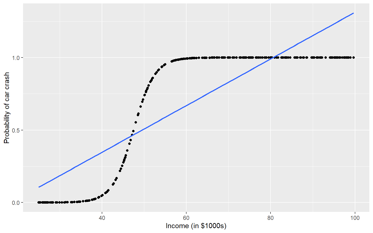
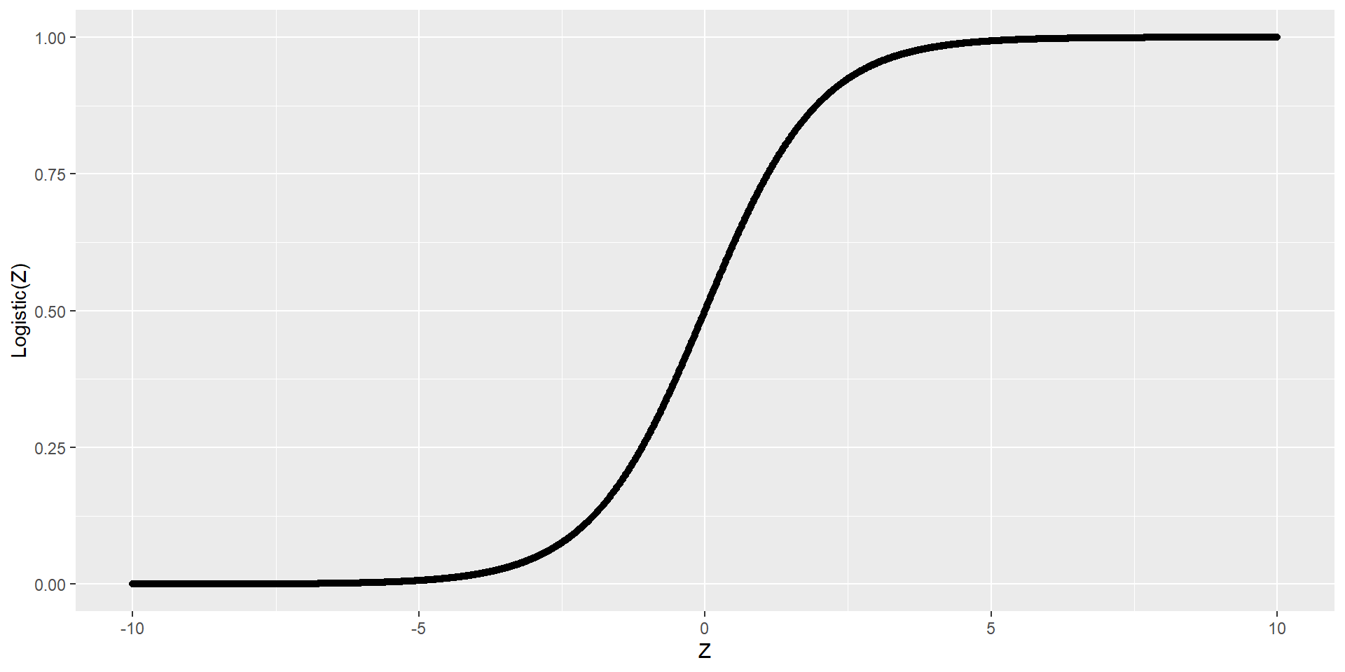
\[\log(\frac{\pi}{1 - \pi}) = \beta_0 + \beta_1 X_1 + ... + \beta_{p-1} X_{p-1}\] Now we have a model that connects \(E[Y|X] = \pi\) to our data, but how do we interpret the parameters, \(\beta_j\)’s?

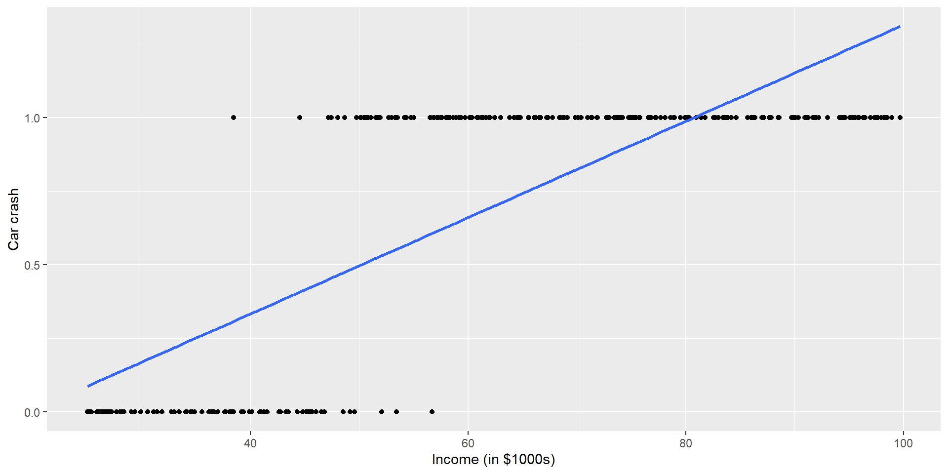
Recall for linear regression: \(E[Y|X] = \beta_0 + \beta_1 X\)

Parameter Interpretation: Solving for \(\beta_1\)

\[\log(\frac{E[Y_i|X_i]}{1 - E[Y_i|X_i]}) = \beta_0 + \beta_1 X_i\]

Parameter Interpretation: Explaining \(\beta_1\)

Odds Ratio

\(e^{\beta_1} = \frac{\pi_a}{1-\pi_a} / \frac{\pi_b}{1-\pi_b}\)

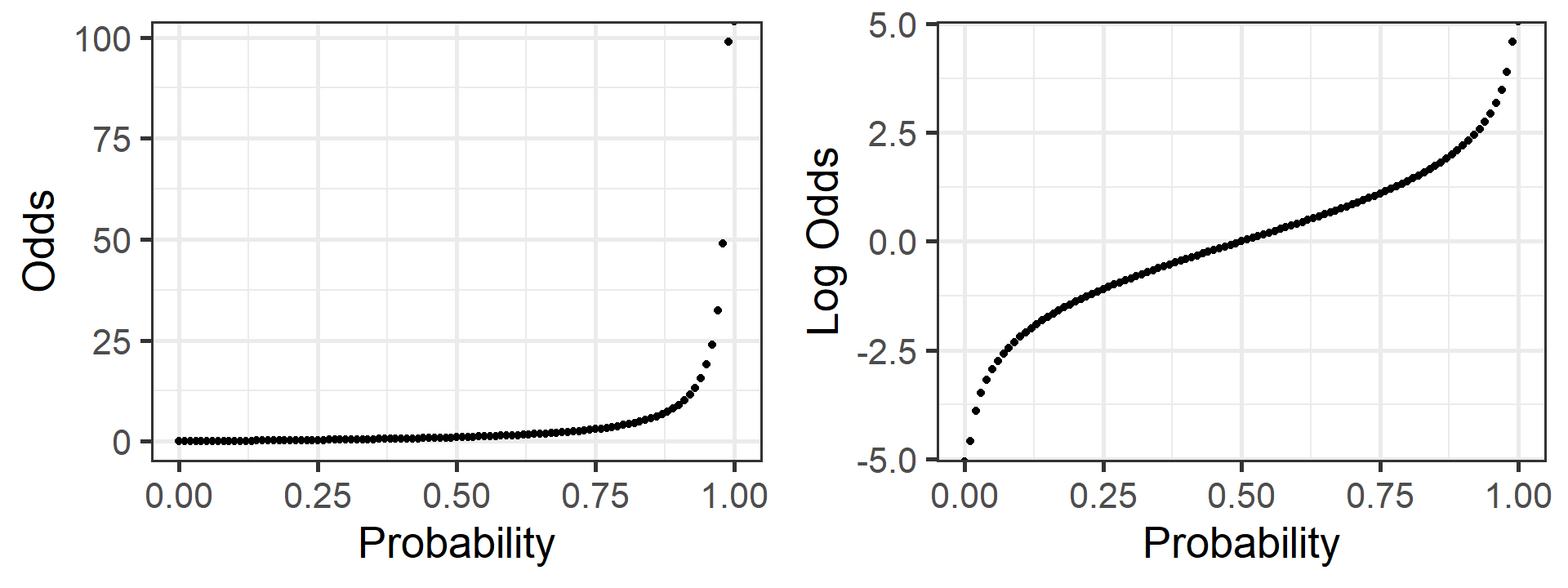
We typically interpret the odds ratio \(e^{\beta_1}\) instead of log odds ratio \(\beta_1\)


If \(e^{\beta_1}\) = 1


If \(e^{\beta_1}\) < 1


If \(e^{\beta_1}\) > 1

Parameter Estimation: MLE

We want the Maximum Likelihood Estimate (MLE) for the \(\beta_j\)’s… why?

  • The MLE aims to find estimates \(\hat{\theta} = \{\hat{\beta}_0, \hat{\beta}_1, ..., \hat{\beta}_{p-1}\}\) that maximize the likelihood function over the parameter space with a given data set.

  • The likelihood function \(L(\theta | y)\) measures the goodness of fit of a statistical model to a sample of data for given values of the unknown parameters \(\theta\).

  • The Maximum Likelihood Estimators have desirable asymptotic (large sample size) properties

Parameter Estimation: MLE for Logistic Regression

We want to find estimators \(\hat{\beta_0}, \hat{\beta_1}, ..., \hat{\beta_p}\) that maximize \(L(\theta | y)\)

  • For simple linear regression we can directly solve for the maximum likelihood estimators and they happen to be identical to the least square estimators
  • For logistic regression we can’t directly calculate the estimators, we have to use optimization algorithms. Luckily those are implemented for us!

Inference With Logistic Regression

In linear regression we used a t-test to test for statistically significant features.

Beware in logistic regression there are different tests that can be used (we will talk about these)

  • Likelihood Ratio Test
  • Wald Test

Know which one your software is using!

Classification / Prediction With Logisitic Regression

How do we convert the predicted probabilities to values of \(Y\) (e.g., 0 vs 1 or TRUE vs FALSE)?

The cutoff should be a domain knowledge-based decision. The natural cutoff with no context would be 0.5

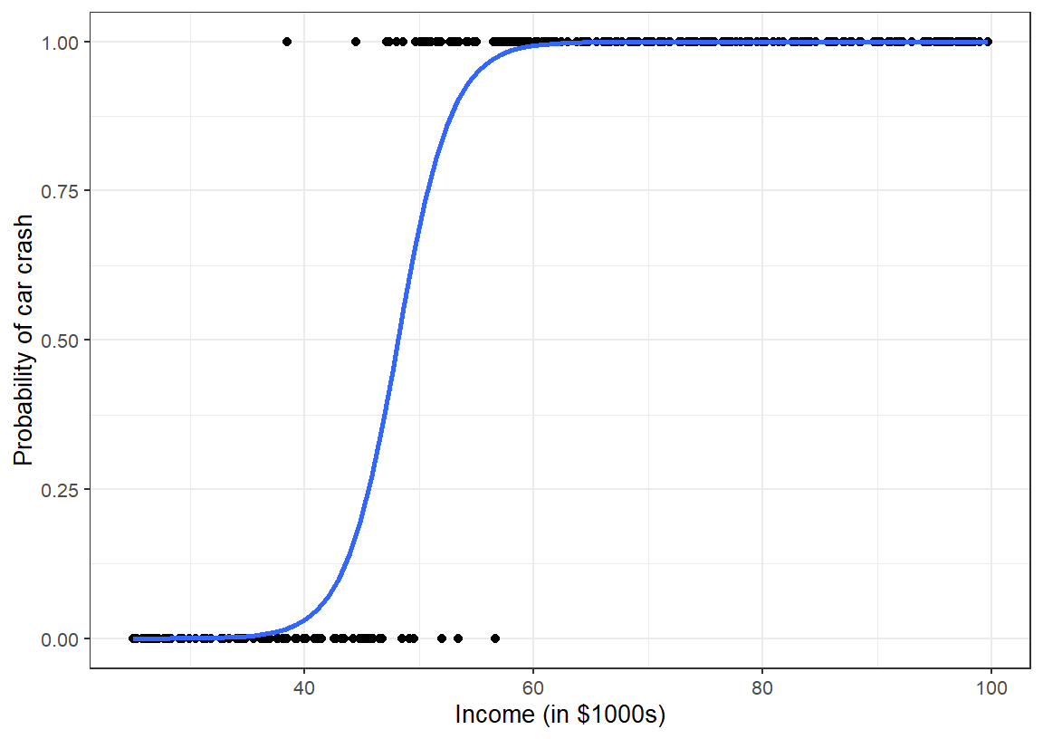
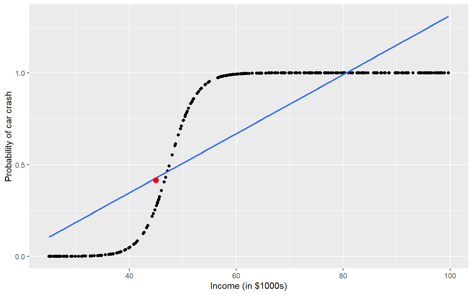
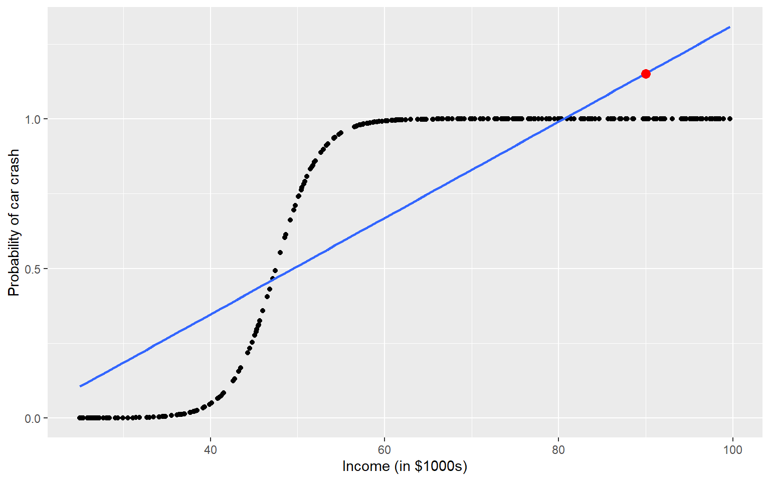
ggplot(sim_crash_data, aes(y = car_crash, x = income)) +
    geom_point() +
    geom_smooth(
      method = glm, 
      se = FALSE, 
      method.args = list(family = "binomial")
    ) +
    theme_bw(base_size = 10) + 
    labs(y = "Probability of car crash", x = "Income (in $1000s)")

Classification / Prediction With Logisitic Regression

Confusion Matrix

There are many considerations for how “well” our logistic model is predicting