Math 430: Lecture 9a
Logistic regression for prediction
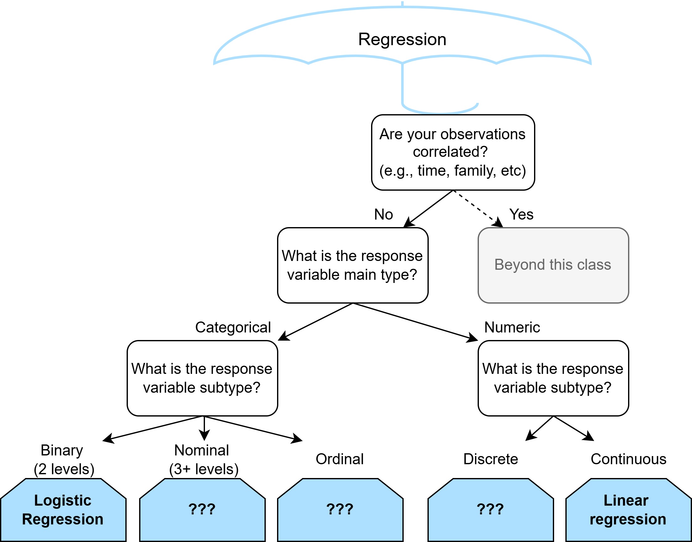
Prediction
How do we decide if our logistic model is predicting well?
Confusion Matrix

Confusion Matrix
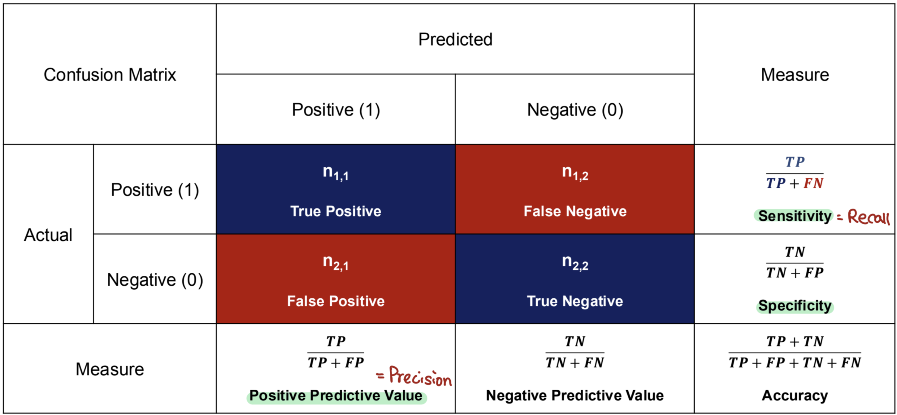
Confusion Matrix: Sensitivity
1.) Sensitivity (= Recall, True Positive Rate)
- TP + FN = # of actual ____________
- How well does the model classify/predict the positive value among the actual positive samples?
- How well does the model detect positive samples accurately?
- Example: Detecting spam emails
- What percentage of spam emails does the model detect among the actual spam emails?
Confusion Matrix: Specificity
2.) Specificity (= Selectivity, True Negative Rate)
- TN + FP = # of actual _______________
- How well does the model classify/predict the negative value among the actual negative samples?
- How well does the model eliminate negative samples accurately?
- Example: Detecting spam emails
- What percentage of non-spam emails does the model detect among the actual non-spam emails?
Confusion Matrix: Trade-off
3.) Trade-off between sensitivity and specificity
- “Best model” = high sensitivity & high specificity \(\rightarrow\) F1-score
- F1-score is bounded between 0 and 1
\[\begin{equation*} \begin{split} \text{F1-score} &= \frac{2}{Precision^{-1} + Recall^{-1}}\\ &= \frac{2TP}{2TP + FP + FN} \end{split} \end{equation*}\]
Recall the Coronary Heart Disease data
Computing confusion matrix
First compute the predictions for each observation.
Next we compute the confusion matrix for our in-sample predictions, this is different from out-of-sample predictions where we would check our predictive performance on new data.
Computing confusion matrix
library(caret)

confusionMatrix(
  as.factor(predicted_chd), # Predicted response
  as.factor(heart_data$chd) # Actual response (from our data)
)
Confusion Matrix and Statistics
Reference
Prediction 0 1
0 258 85
1 44 75
Accuracy : 0.7208
95% CI : (0.6775, 0.7612)
No Information Rate : 0.6537
P-Value [Acc > NIR] : 0.0012297
Kappa : 0.3438
Mcnemar's Test P-Value : 0.0004286
Sensitivity : 0.8543
Specificity : 0.4688
Pos Pred Value : 0.7522
Neg Pred Value : 0.6303
Prevalence : 0.6537
Detection Rate : 0.5584
Detection Prevalence : 0.7424
Balanced Accuracy : 0.6615
'Positive' Class : 0
Computing F-1 score
Are there other ways to define “best model”?
Maybe a few…
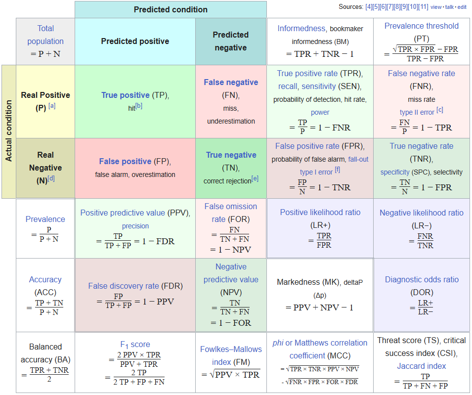
https://en.wikipedia.org/wiki/F-score
When you encounter a new evaluation metric some good considerations are:
- What constitutes a “good score”? Is the score bounded?
- What is being valued? E.g., TP? FN?
- Does it match what I value in this context?
- E.g., When predicting cancer maybe we are more concerned with _____
- E.g., When predicting mechanical failure and considering hiring an additional mechanic in a warehouse we might be more concerned with ______
Other models for binary classification
Recall
We chose the logistic function to link our expected response to our linear model
\[logistic(Z) = \frac{e^z}{1 + e^z}\]
\[E[Y_i | X_{1i}, ..., X_{pi}] = \frac{e^{\beta_0 + \beta_1 X_{1i} + ... + \beta_p X_{pi}}}{1 + e^{\beta_0 + \beta_1 X_{1i} + ... + \beta_p X_{pi}}}\]
\[log(\frac{E[Y_i | X_{1i}, ..., X_{pi}]}{1 - E[Y_i | X_{1i}, ..., X_{pi}]}) = \beta_0 + \beta_1 X_{1i} + ... + \beta_p X_{pi}\]
Link
We chose the logistic function to link our expected response to our linear model
\[E[Y_i | X_{1i}, ..., X_{pi}] = \frac{e^{\beta_0 + \beta_1 X_{1i} + ... + \beta_p X_{pi}}}{1 + e^{\beta_0 + \beta_1 X_{1i} + ... + \beta_p X_{pi}}}\]
We liked this link function because
- It was bounded between 0 and 1
- It results in odds interpretation for coefficients
What other link functions, aside from the logistic link, could we have used?
Probit regression
One possible link function that is also bounded between 0 and 1 is the probit link
\[E[Y_i | X_{1i}, ..., X_{pi}] = \Phi(\beta_0 + \beta_1 X_{1i} + ... + \beta_p X_{pi}),\]
Where \(\Phi( \cdot )\) is the cumulative standard normal distribution function.
Con: \(\beta_j\) does not have a simple interpretation
Call:
glm(formula = chd ~ sbp + famhist + age, family = binomial(link = "probit"),
    data = heart_data)

Coefficients:
                Estimate Std. Error z value Pr(>|z|)
(Intercept)    -2.674195   0.449235  -5.953 2.64e-09 ***
sbp             0.003769   0.003267   1.154    0.249
famhistPresent  0.559544   0.130075   4.302 1.69e-05 ***
age             0.033541   0.005290   6.340 2.29e-10 ***
---
Signif. codes:  0 '***' 0.001 '**' 0.01 '*' 0.05 '.' 0.1 ' ' 1

(Dispersion parameter for binomial family taken to be 1)

    Null deviance: 596.11  on 461  degrees of freedom
Residual deviance: 504.94  on 458  degrees of freedom
AIC: 512.94

Number of Fisher Scoring iterations: 4
logistic_pi_predictions <- predict(heart_logistic_model, newdata = heart_data)
logistic_y_predictions <- ifelse(logistic_pi_predictions > 0.5, yes = 1, no = 0)
probit_pi_predictions <- predict(heart_probit_model, newdata = heart_data)
probit_y_predictions <- ifelse(probit_pi_predictions > 0.5, yes = 1, no = 0)Confusion Matrix and Statistics
Reference
Prediction 0 1
0 284 121
1 18 39
Accuracy : 0.6991
95% CI : (0.6551, 0.7406)
No Information Rate : 0.6537
P-Value [Acc > NIR] : 0.02163
Kappa : 0.217
Mcnemar's Test P-Value : < 2e-16
Sensitivity : 0.9404
Specificity : 0.2437
Pos Pred Value : 0.7012
Neg Pred Value : 0.6842
Prevalence : 0.6537
Detection Rate : 0.6147
Detection Prevalence : 0.8766
Balanced Accuracy : 0.5921
'Positive' Class : 0
Confusion Matrix and Statistics

          Reference
Prediction   0   1
         0 297 144
         1   5  16

               Accuracy : 0.6775
                 95% CI : (0.6327, 0.7199)
    No Information Rate : 0.6537
    P-Value [Acc > NIR] : 0.1522

                  Kappa : 0.1049

 Mcnemar's Test P-Value : <2e-16

            Sensitivity : 0.9834
            Specificity : 0.1000
         Pos Pred Value : 0.6735
         Neg Pred Value : 0.7619
             Prevalence : 0.6537
         Detection Rate : 0.6429
   Detection Prevalence : 0.9545
      Balanced Accuracy : 0.5417

       'Positive' Class : 0